Reference material for Omniscope beyond that available in the video tutorials [1].
Please use the index on the left to navigate.
Omniscope version 2.5 offers 16 different views. More views are always under development. You can preview/test experimental views available in your version at any time by enabling experimental features on your installation, then re-start your Omniscope: Version 2.5: Settings > Advanced > Show experimental features
View Toolbar [2] - documentation of View Toolbar commands and options common to all views | |||
Table View [3] - see all of your data in rows and columns, with aggregation options, grouping for sub-totals, formulae and variables for modelling, and a wide range of powerful data editing tools. | |||
| Chart View [4] - horizontal visualisations of data values in your columns, a powerful view for querying ranges and spotting errors your data. | ||
Pie View [5] - show splits/proportions of values in category, number and date fields, with paning for multiple pies per view. | |||
| Bar View [6] - display relative levels in multiple category, numeric or data fields using horizontal, vertical, stacked, cascaded and proportional bars. | ||
| Graph View [7] - identify relationships between columns with scatter plots or time series [8], using statistical analysis to identify trends, outliers and exceptions. | ||
| Tile View [9] - Show each record as a re-sizable tile or image,useful for 'heat maps', image catalogues and much more. | ||
| Pivot View [10] - displays summary values (sums, means, counts, etc.) at intersections of selected category columns. | ||
| Network View [11] - depict both grouped hierarchies and relational networks using either dual field or specified multi-field relatonships. Grouped networks can be used to visualise almost any type of data set, while relational networks can be used whenever there is a common relationship between the rows. | ||
| Portal View [12] - text search plus dynamic filtering of categories, numbers and dates and statistical summaries of the target universe. | ||
| Map View [13] - geo-spatial positioning of records, with embedded or web-based maps enabling selection, filtering, and connected markers. [14] | ||
| Venn View [15] - See the overlaps between up to 5 pre-defined subsets of the data ('named queries') corresponding to the filter settings or selections in place at the time you save or add to the named query. | ||
| Web View [16] - use multiple web views to display multiple web pages, and exchange data with remote web services. [17] | ||
Content View [18] - place formatted text annotations with embedded images and formulas in this view window located anywhere on the page. (new in 2.5) | |||
Dial View [19] - adds dial and meter type visualisations with defined alerts and zones for high-impact dashboards. (new in 2.5) | |||
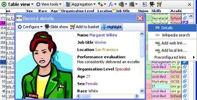
| Details View [20] - see some or all the displayed attributes of each record, with associated image(s) and links. | ||
This section covers the View Toolbar commands which are common to all views. Documentation for view-specific commands on the View Toolbar > View Tools menus of each view are discussed view-by-view in the Views Reference [21] section.
![]()
Every View has a View Toolbar at the top. The View chooser, Data Subset query selector, Aggregation options, View Tools, Fields chooser, show Details and [X] Close View button at the far right end are present on most View Toolbars. Exceptions: Details View only shows the details for a single record, the Web and Content Views.
![]() View Chooser - the selected view name and icon always appear at the far left of the View Toolbar. Click on the drop-down View Chooser to change the view displayed in the window.
View Chooser - the selected view name and icon always appear at the far left of the View Toolbar. Click on the drop-down View Chooser to change the view displayed in the window.
![]() Data Subset - the data set or filtered/defined subset to be displayed is selected here. By default, the Filtered data (IN) subset is selected. If no filters are set, this will be the same as All Data. If you have defined Named Queries [22], they will be added to the bottom of this menu in each view.
Data Subset - the data set or filtered/defined subset to be displayed is selected here. By default, the Filtered data (IN) subset is selected. If no filters are set, this will be the same as All Data. If you have defined Named Queries [22], they will be added to the bottom of this menu in each view.
![]() Aggregation - most views enable you to select various options for defining and visualising aggregated data sets, and specifying the functions to be applied to each field (column) in the aggregated displays. For more detail, see the section on Aggregation & Grouping.
Aggregation - most views enable you to select various options for defining and visualising aggregated data sets, and specifying the functions to be applied to each field (column) in the aggregated displays. For more detail, see the section on Aggregation & Grouping.
![]() View Tools - drop-down menu present on all View Toolbars, but most of the commands on this menu differ by view. The commands which are common to almost all views are discussed below. View-specific commands are discussed in the section on using each view.
View Tools - drop-down menu present on all View Toolbars, but most of the commands on this menu differ by view. The commands which are common to almost all views are discussed below. View-specific commands are discussed in the section on using each view.
![]()
Fields - you can choose the fields (columns) displayed or hidden, and the order in which the columns are displayed on a view window-basis. Use the 'All' or 'None' buttons to show or hide all columns, and change the order by dragging the 'hands' up or down to order the columns.
![]()
Details - This button, next to right-most in all View Toolbars, displays a pop-up table (with the same settings as the Table View) showing all records currently visible in the view. If you have made an active selection before clicking on Details, you will be asked if you want to display only the selected records. The first column in the pop-up table will have underlined values, which are links to the individual records. Click on the underlined record to display that single record in a Details window. Alternatively, double-click the row number ("row header") to see the details for a record. For more detail, see Viewing Details. [23]
![]() Close View - clicking on this icon will close each individual view.
Close View - clicking on this icon will close each individual view.
![]() You can re-open/return to a given view at any time using the Add View chooser drop-down from the Main Toolbar:
You can re-open/return to a given view at any time using the Add View chooser drop-down from the Main Toolbar:
This discussion of the View Toolbar > View tools drop-down menu covers only those commands common to all or most views. Most of the commands under View Tools are specific to each view. These commands are discussed in the sections on each view, accessible for the links on the Views Reference [21] page.
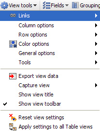
The bottom-most section of commands in the View Tools drop-down menu is the same for all views:
Background image - see discussion below
Export view data - takes you to the Export Data wizard (also accessible from the Main Toolbar File > Export > Export files menu). Opening the Export Data wizard using the View Toolbar > View Tools > Export view data command pre-selects the data set of the current view as the set/subset of data to be exported. The Export Data wizard allows you to add or remove fields from the file to be exported, set the column order to match the view and to decide which export file format to use, either .IOK or .CSV or Excel .XLS for spreadsheets, or .XML for other applications).
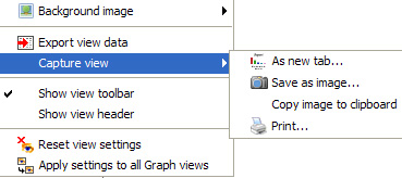
Capture view - provides 4 options for capturing the visible aspects of each individual view:
Show view toolbar - this option determines whether the View Toolbar is revealed or hidden. When creating report tabs, for example, it is often desirable to hide the View Toolbar if users do not need to alter the view settings. If you have saved the tab in default format the View Toolbar will be hidden...to reveal it for just one one view, say a Web View, tick this option.
Show view header - this option reveals an editable text title space above the View Toolbar each view
Reset view settings - allows you to reinstate the default settings for the view if you have changed the row heights, field order, etc.
Apply these settings to all {view name} views- extends the settings you have configured for the view to all other views of the same kind. For example, if you have set a particular column order for a Table View, this command copies the settings to all other Table Views you have configured thus far. If you have configured Table Views in saved report tabs, you will be asked if you want to change those settings as well.
The Pie, Bar, Graph, Portal and Details View Toolbar menus also contain the option to specify an image to be shown as a background to the view.
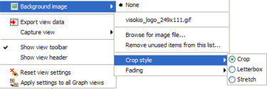
Image files such as logos, etc. of any size in .JPG or GIF format can be added as background, sized to fit using the Crop, Letterbox or Stretch options, then faded to create an unobtrusive backdrop for selected views. For more on working with background images, see the section on the Layout Menu [25].
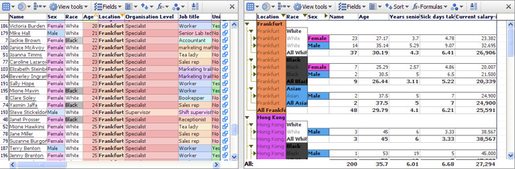
The Table View displays your tabular data as it was imported into Omniscope from a spreadsheet tab or a database view/table. The Table View shows the underlying data values by row and column cells for selection, sorting and editing. Double or right-clicking on a cell allows you to edit the contents, and you can import large tables of data from other sources by cutting and pasting the data into the Table View. The Table View displays colour-coded values with instant aggregation and sorting, plus displays of zooming views of images associated with the data set.
Like spreadsheets, you can specify formula fields (columns) calculated according to formulae you specify using values in other fields (columns). Each record (row) also has a links menu on the row footer (far right end of the row) enabling you to insert dynamically-generated local and web links, or select from a menu of pre-configured links to free web services. Use the View Tools menu commands to check for duplicates, expand and collapse text values into more or fewer columns, and many other data management and correction tasks.
The Table View is highly-configurable, enabling you to drag columns to re-order. To hide (not delete) a field (column), right-click on the column header, select the Tools sub-menu, and select Hide from this view. The Reset all settings for this Table View command at the bottom of the View Tools menu restores all columns to the view, resets the column order to the original import order, and clears all record sorts, aggregations and colouring options. It does not affect Formula field or variable declarations.
The Table View control menus are available via left and right-clicks on the column and row headers, and right clicking on individual cells. These menus are discussed below.
Left clicking on column headers places a primary sort on the data set using the values in that column, and clicking again reverses the sort direction. Small orange triangles pointing up or down indicate that an ascending or descending sort has been set using the values in a column. The primary sort column triangle is solid orange, the other secondary sorts are unfilled. To see or clear sorts that have been set, use the Sorted Fields by Priority drop-down on the View Toolbar (see below).
Sorting-sets the primary sort for the display ascending/descending on values in the field (column). You can remove a sort on this menu, or change the order or direction of sorts. To see and manage all sorts, use the Sorted Fields by Priority drop-down on the View Toolbar (see below).
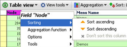
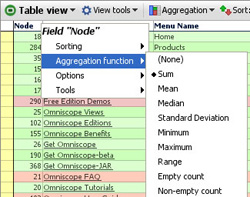
Aggregation function- When you have Aggregation set, the function to be applied to the record (row) values taken collectively for each filed (column) can be different field by field. The aggregation functions available on each column header sub-menu will depend on the data type of the field (column). For example, text columns minimum and maximum values are based on character counts. Note: Range gives the difference between the minimum and maximum values in the field. (See Table View > View Toolbar > Aggregation below for more on configuring aggregation.)
Options- You can choose to display related image sets in any column, or to display configured links, either to the details display of the record, or another link you have configured using the Settings > Links wizard on the Main Toolbar.
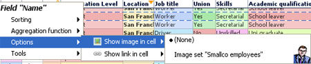
Show image in cell- allows you to insert an image into each cell of a column, regardless of the value in that cell. Choose from the list of image sets which you have previously configured using Settings > Images wizard on the Main Toolbar. Multiple image sets can be displayed this way since several columns can show different or the same images.
Show link in cell- this option will display a sub-menu of links to display when the value in the column cell is clicked. You can link the values in any column to either the Details display, or other links which have been configured for the file using Settings > Links wizard on the Main Toolbar. You can link the values in more than one cell to the same link, or the Details display.
Tools- these column header sub-menu options mirror those available in the bottom section of the View Tools drop-down menu (documented in the View Tools section below). Some of these options (Hide, Rename, Convert field data type, Field options, etc.) mirror those available in Data > Manage Fields on the Main Toolbar documented here [26].
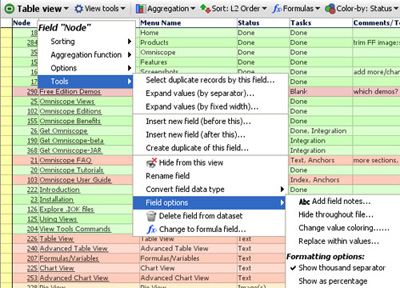
Warning: When using the Expand values commands, you need to create new, blank columns adjacent to the column being expanded to receive the separated values. If you do not, you will be warned about values in the adjacent columns being overwritten. Create new blank target columns and drag them into position to the right of the column to be expanded using Data > Manage Fields > Add new field (at the bottom). See more discussion of using the expand and collapse commands under View Tools commands below.
Warning: Be careful when converting the field data type, as this will delete all non-compatible cell values in the field (e.g. text values will be deleted from a field converted to number field). see more discussion of changing field data types in Data > Manage Fields [26] menu section.
Change to formula field- changes a non-formula field to a formula field. Any values in the column will be replaced by calculated results.
Convert to static values- changes a formula field with calculated values to an input colmun with static values, which you can overwrite. All formula logic will be lost.
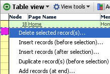
The rectangular space at the far left of each row is called the row header. Left clicking on the row header selects the row, such that you can apply power query filtering operations like Move or Keep to exclude or focus on that record (row). Double-clicking on the row header brings up the Details display. Right-clicking on the row header displays a menu of options for managing the rows in the data set:
Note: If you have sorting or aggregations set, you may not see new blank rows where you expect them. Often it is best to clear all sorts and aggregations when adding or deleting rows.
The rectangular space at the far right of each row is called the row footer. Left or right-clicking on the row footer displays a Links menu which allows you to follow or define additional links using the Add web or local links wizards also accessible from Settings > Links on the Main Toolbar.
Right-clicking on an individual cell displays a selection and viewing options sub-menu:
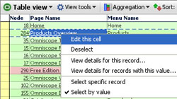
Edit this cell- is the same as double clicking on the cell to place the cursor inside the cell.
Deselect- removes this record from the selection set. This is not the same as the global Deselect on the the Main Toolbar which removes all records from the selection set.
View details for this record- displays the individual record Details for the selected record.
View details for records with this value- launches the pop-up table view containing all records which share the same value in the cell. The pop-up table view will be configured the same as the Table View you clicked on in terms of column order, columns displayed etc.
Select specific record- Use carefully!...when ticked, this changes the selection behaviour to select records one at a time, rather than based on common values. If this option is ticked IT APPLIES TO ALL fields (columns). When ticked, the Main Toolbar barometer will only show 1 record selected at a time, unless you drag the mouse to select contiguous records. Resetting the the Table View returns this setting to the default Select by value.
Select by value- the default behavior...if you select a cell, all records that share the same value in that cell are selected, as shown in the Main Toolbar barometer in blue. You can then execute power queries such as Moves and Keeps on the selected records.
The Table View Toolbar contains 5 view specific drop down menus; View Tools, Aggregation, Sort, Formulas, Colour-by: and Colour Options in addition to the View Chooser and the Show Details, Add to Basket and [X] Close window icons common to all views:
![]()
Each of these sections is documented below:
The Table View tools menu has six sub-menus; Links, Column Option, Row Options, General Options, Aggregation and Tools. The sections below document the commands and options available under each of these sub-menus.
The Links sub-menu enables you to select which, if any, links will be associated with clicking on the values in the cells of each field (column) in the Table View.

Fields already associated with links will show on the drop down list in bold, and their values underlined in the cells of the Table View to indicate a live link.
No links (None) is the default for all fields except the first column on first opening, which is set to Details (which you can change). Any number of different fields can be linked to the Details display. All other links which you have configured for the file (using the Settings > Links menu on the Main Toolbar) will show on the pick list, available for association with any of the fields in the data set.
The Column options sub-menu enables you to choose which fields (columns) will be shown or hidden (not deleted), and the order in which they will be displayed for that particular Table View (global column order for the file is set at import, but can be changed using Data > Manage fields on the Main Toolbar).

Columns to show- reveals a list of all fields which are ticked (showing) or unticked (hidden) in this Table View. Tick or untick the check boxes to show or hide columns and/or drag the hands up or down to change the order of columns. You can also click and drag the column headers sideways to reorder the columns, and you can hide columns by right-clicking the column header, then selecting Tools > Hide from this view. Suggestion: use the ALL or NONE buttons at the top right of the Columns pick list to reset the columns displayed quickly.
Column header height- allows you to add more lines to column headers to accommodate longer names on narrower columns.
Squeeze columns (prevent scrolling)- turns the column header text vertical (if necessary) and narrows all the columns/cells to display in the window available with a minimum of horizontal scrolling. Cell values are concatenated by default, but full cell contents will show as the mouse hovers over the cell.
Reset column widths- (not shown when Squeeze columns is ticked)- resets the display of the columns on display based on the space available and number of columns being displayed. Columns can be widened or narrowed by dragging the edges of the column headers. This command provides a reset to defaults.
Note: The settings that you make for a given Table View will not be applied to the Show details pop-up table unless you also choose Apply these settings to all Table Views.
The Row options sub-menu is used to manage the display of records (rows)
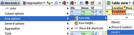
Row title- can be used to select a value to display in the row header. The default is the record number assigned by Omniscope, but if there is a more meaningful identifier in the data set, you can choose to display it instead. Alternatively, you can choose (None) and the row header will be narrow and blank.
Row height- used to increase the number of lines in a row. The default is one, but if you wish to display images in cells, you may want to increase the number of lines using the slider. Display an image in one column, then increase the row height and width of the column. The images will expand to fill the space and the text will wrap.
Show link shortcuts- by default, shortcuts to the various configured links are accessible from an icon on the row footer at the far right of each row. Unticking this option hides the row footer, which may not be needed by file users and frees up a small amount of horizontal space.
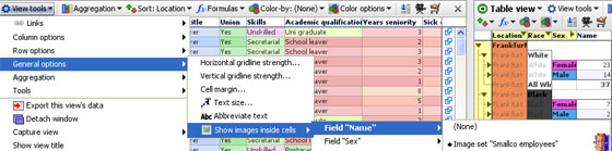
The General options sub-menu contains options related to cell display.
Horizontal/Vertical gridline strength- removes or emboldens the lines defining the rows, columns and cells.
Cell margin- increases the white space around the edges of the cells from the default of none, to as much as 10 pixels. Can improve legibility, especially if used in conjunction with increased text size (see below)
Text Size- increases the size of the font used in the headers and cells of this Table View.
Abbreviate text- allows you to turn on and off cell text abbreviation. Abbreviation is useful when cells contain long text.. making columns too wide. With abbreviation turned on, you will still see what the cell contains in a much smaller space. Abbreviation is turned on by default.
Show images inside cells- allows you to chose an associated image set to display as a zooming image in a particular field (column). Note: the images will obscure the underlying values, so it is best to use a column containing the image references, which are often cryptic image file names, or else a blank column added specifically for the purpose of displaying the images.
The Tools sub-menu provides some powerful functions to manage the format and layout and otherwise improve the quality of your data sets.
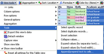 |  |
Select specific record- turns off the default common value-based selection i.e. clicking on any cell selects only the record that contains that cell rather than all the records sharing that value in the field (column). This makes the table behave a bit more like a spreadsheet and enables you to select rows to Move, Keep or Add to the Basket individually.
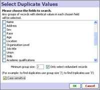
Select duplicate records- displays the Select Duplicate Values wizard that for selected fields, isolates all records that have more than one identical value elsewhere in that field (also works for multiple fields). This is useful for eliminating duplicate records in large datasets. The Select Duplicate Values wizard allows you to select which fields to check for duplicates, or triplicates etc. If you select more than one field (column) then records duplicated in either column (but necessarily both) will be selected.
Minimum group size: use the value of 2 to detect duplicates (or triplicates); use the value 3 to detect triplicates but not duplicates
Only select redundant records- once processing is completed, the default is to leave all rows containing duplicates (or higher) selected. If you tick this option, the first duplicated record will not be selected, so that you can you can perform Moves to eliminate only the redundant records, and Add to Baskets to create correction files.
Case sensitive- requires duplicated values to match case in order to be considered duplicates.
Invert selection- If you have selected a complex pattern of records, and wish to quickly select all other records not currently selected, use this command.
Collapse values- used to combine some of all of the values currently in more than one column into a single column, with a space or some other separator you specify in between the values. You must have selected a range of columns and rows to collapse before clicking on this command. Used to reduce column count and to create tokenized fields, which contain more than one value per cell and are used to to capture many-to-one relationships in tabular data. For more information, see Tokenized Data [27].
Note: You cannot select a group of columns using the column headers. To select all or part of a range of columns, select the first cell in the first column, then drag the mouse across to the right to select more columns and downward to select more rows. If you need to select many more rows than are visible, hold the Shift key and use the vertical scroll bar to bring the bottom right hand cell of your range into view. Click on that cell with the Shift key still depressed and the entire rectangle of columns and rows will be selected.
Expand values (by separator text)- used to replace a single column of data containing compound elements (e.g. First and Last Name with a space between) with multiple columns each containing a single element, such as First Name Column and Last Name Column. Before using this command, you must select the compound (separated value) column you wish to expand and create new blank column(s) adjacent to the right of that column. Be sure to select the entire column to be expanded using the Shift + scroll down method to ensure you have selected all the way to the bottom of the column- assuming the expansion should include all the cells in the column. Click on the command and you will be asked to specify the text separator defining the elements to be expanded, such as a blank space, which must be entered.
Note: create the new, blank columns using the Data > Manage Fields > Add new field button (at the bottom) then drag the new column into place below (right of) the column to be expanded, making sure to tick the new column in the Columns to show list of you are in Reports Mode. The existing column will be used for the first element, so to split two elements you need only add one new column.
Expand values (by fixed width)- used to break a single column of data into more than one column based on defined break points you set using the Expand Values wizard:
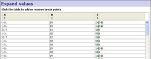
Before using this command, you must select the column of values you wish to expand and create sufficient new blank column(s) adjacent to the right of that column. Be sure to select the entire column to be expanded using the Shift + scroll down method to ensure you have selected the column all the way to the bottom - assuming the expansion should include all the cells in the column.
Append/prepend to cells- used to add specified characters before or after the existing values in the cells.
Note: sometimes when exporting numeric identifiers with leading zeros to Excel, such as Bloomberg Excel spreadsheets using SEDOLs, Excel does not recognise the incoming values as text and drops the leading zero, rendering the identifier incomplete. To stop this, use the Prepend function to add a text character such as an apostrophe ' in front of the numeric identifiers to force Excel to treat the values as text.
The Aggregation sub-menu controls the display when aggregation is set for a given Table View. Aggregation groups rows together based on common values. You specify the fields (columns) on which aggregation is based in sequence. For example, if you have a data set in which each record (row) is a person, you might choose a Table View display which aggregates the rows first by Location, and then by the values in other fields, like Race or Sex (grouping the males and females in each location). You set the aggregation sequence using the Aggregation pick list on the View Toolbar. If you have more than one aggregation set, use the hands to drag aggregated fields into the order in which you want the aggregations presented top to bottom = from left to right.
Note: Many different aggregation functions are availabe, and they can be different for each column. Right-click on the column header to see which aggregation function is specified for each column in the Table View.
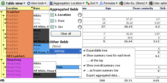
Expandable tree- when ticked, displays a navigational 'tree' in the far left row header. Clicking on the black triangular arrows either expands or collapses the view of the rows at a particular level of aggregation.
Show summary rows for each level- when ticked, displays a summary row for each aggregated set of rows. The summary row calculates a value based on the function you select in each column by right-clicking on the column header and selecting the aggregation function to be used for that column.
...at the top- when ticked, displays the summary row for each set of aggregated rows at the top of the grouping rather than at the bottom
Show overall summary row- when ticked, shows a summary row for all rows, using the function specified for each column by right-clicking on the column header and selecting the aggregation function to be used for that column.
...as frozen summary row- when ticked, keeps the overall summary row visible at the bottom of the Table View window.
Export aggregated data... creates a new .IOK file where the rows reflect the values selected for aggregated rows in the source file.
Sorting for each Table View is set using the Sort drop-down menu. Tick the check box of any field to sort the table by this field. Click the orange arrow next to each field name to reverse the direction of the sort. Drag the hands next to each field to change the order of primary, secondary and subsequent sorts.
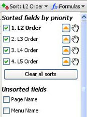
Use the Clear all sorts button to remove all sorts from this Table View. Note: It is common to set sorts accidently by clicking on column headers. Always keep an eye on the Sort: field to ensure you have not inadvertently added a primary sort at the top of the list. If you have, simply untick the unwanted sort on this list and it will be removed...no need to use Clear all sorts.
Omniscope can calculate values based on values in other columns, using a standard menu of functions (plus some additional Visokio DATASET functions) and the same syntax as Excel.
![]()
Add formula field- creates a new field (column) of values calculated as a function of the values found in other columns, together with any variables whose ranges have been defined (see discussion of variables below). Use the Add formula field wizard to define the calculation you want Omniscope to perform when populating the new column. For more detail on using the Add formula wizard, see the section on Formulas and Variables [28].

Convert existing field to use formula- use this command to substitute any values that may be in an existing column with calculated values based on a formula you specify using the Add formula field wizard.
Edit formula- allows you to select the already-defined formula you want to edit, and displays the current formula definition in the Add/Edit formula field wizard for editing. Formulae are specified by selecting columns and typing in arithmetic operators and selecting functions from the the functions library. The functions library contains all the standard spreadsheet functions, plus special Visokio DATASET functions documented in the Functions Guide [29]. For more detail on using the Edit formula wizard, see the section on Formulas and Variables [28].
Formula calculations and aggregation options (see below) can interact. The precedence settings determine (for each Table View) whether the fields with formulae defined are calculated at individual record level, then aggregated, or aggregated first:
Calculate aggregated values over formula field results- the default behaviour (aggregation of row values happens after formulae are calculated)
Calculate formula field results for aggregated values- this option changes the precedence of the calculations, such that a formula such as =[USD Volume] / [Deal Count] in an aggregated table using aggregation function Sum, is evaluated as Sum (USD Volume) / Sum (Deal Count) for the aggregate rows. Notice that with this option set, two "sum" concepts at play: inside a formula, SUM(Column A, Column B, Column C...) calculates the SUM of multiple fields within the same row. In the aggregated table, the aggregation function Sum calculates the vertical sum of all record values within the same field (column) in the aggregated row.
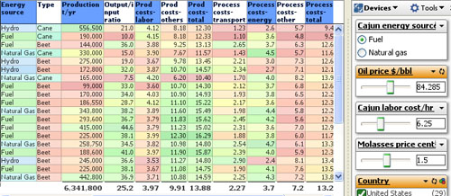
Add/Edit variables: Variables are input assumptions (not fields in the data set) you define by setting a default value and specified upper and lower ranges. Variables are used as flexible input assumption values so that dynamic sensitivity analyses and real-time modelling options will be available to users of the file. If you define Variables, the input values can be set by devices which appear on the Side Bar. These sliders must be visible (ticked in the Devices drop-down menu on the Side Bar) in order for you and your users to 'flex' the assumptions by adjusting the current value of the Variable(s). Any Variable(s) whose current value is different from the default will show an orange device panel, the same as for set filter device panels. For more detail on defining and using variables, see the section on Formulas & Variables [28].
Colour-by: {Field Name} or (None): This drop down menu allows you to select the field (column) by which to colour the rows in the Table View. If you select a field, it overrides the default colouring based on field data type (white for text fields, ranges from red (low) to green (high) for numeric fields, etc.) to colouring that defines records by the value and assigned colours of any any field (column) you select. You can set the colour associated with each category in the field (column) using Data > Manage Fields > Configure > Field Options > Change value order, colours and shapes. You can also access the Field Options command from the Column Header right-click Tools sub-menu shown above.
The Colour Options sub-menu is used to change the colouring behaviour of each Table View.
 | Aggregation group cells- colours the aggregation headers at the left of tables with aggregations set based on the colours assigned to the categories being aggregated. |
Granular record cells - if you find even the unaggregated cell colouring distracting, and want to return to black and white, untick this option to turn colouring off altogether.
Alternate row colour variation- to increase legibility, Omniscope alternates the intensity of colouring in alternating rows. You can strengthen or weaken this effect using the slider displayed by this command.
Text contrast- you can modify the intensity of the text display to suit your display and lighting/presentation conditions
Note: Formulas and variables can be managed from several places, principally the Data > Formulas menu. Please see Formula Fields [30] for a general guide to using formulas and variables in Omniscope.
Grouping options and formula calculation options can interact. In the Table View's Formula menu, two additional options are provided allowing you to configure the precedence of formula calculation when you are Grouping by fields or using Group > Show overall summary row. These precedence settings determine whether fields with formulae defined are calculated at individual record level, or at Grouped level:
Table View: View Toolbar: Formulas > Calculate group result values over formula field results
This is the default behaviour (grouping/summing of row values happens after formulae are calculated). Formulas are calculated for ungrouped data, then the function chosen (e.g. sum) is applied to the formula results, producing the grouped cell value.
Table View: View Toolbar: Formulas > Calculate formula field results for group result values
This option changes the precedence of the calculations, such that a formula such as =[USD Volume] / [Deal Count] in an grouped table using grouping function Sum, is evaluated as Sum(USD Volume) / Sum(Deal Count) for the grouped rows. Notice that with this option set, there are two "sum" concepts at play: inside a formula, SUM (Column A, Column B, Column C...) calculates the SUM of multiple fields within the same row. In the grouped table, the grouping function Sum calculates the vertical sum of all record values within the same field (column) in the grouped row.
Note: some of the now-deprecated Visokio DATASET functions will not work with grouped table rows in this mode. If you use this option, and you have grouped table rows while using certain DATASET functions, you will see "error" in the grouped cells of any formulae using the unsupported functions. For more information on substituting SUBSET functions for the now-deprecated DATASET functions, see the Functions Guide [29] in our KnowledgeBase.
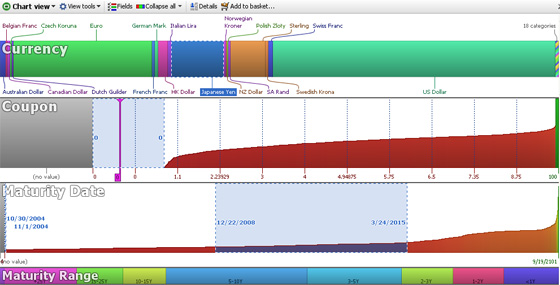
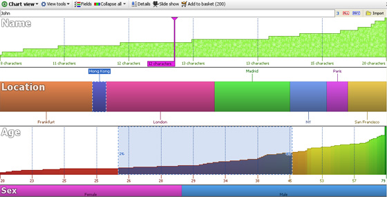
The Chart View gives the most comprehensive overview of the contents and structure of your data sets. In one display, the entire composition of the file is revealed, enabling you to see relative proportions, ranges, gaps in the data, etc.
The Chart View shows all the fields (columns) in the data set as horizontal visualisation bar devices, with continuous values like numbers and dates/times plotted smallest to largest, and category values divided into different coloured segments. Text values are shown in devices coloured in ‘alphabet soup’ where the vertical height indicates the number of characters in each text string. Null/blank values are shown as grey segments. Remember that nulls/blanks are not the same as zero values. Zero values will display as a single coloured line at the bottom of a numeric bar device with a white, rather than grey background. In the example below, the field Coupon is numeric and contains both null and zero values. All of the zero values are selected and one is highlighted:
Text devices for text entries with many different values, such as names, comments etc. the Text visualisation bar devices show a 'staircase' curve based on the number of characters in each value in ascending order left to right. Selection inside Text devices is done in one of two ways; either by text input (keywords- the default) or by clicking and dragging. Right-clicking inside a Text visualisation device will display a menu with the option to set Selection to clicking and dragging. Using this setting, you can select suspicious text records based on blank values, or character counts longer or shorter than you would expect for your identification codes, etc. In the example below, the field 'Name' below displays as a Text device. If we select based on keywords, we can enter 'John' at upper left. Notice at the far right of the device that we found 3 'hits' on the name 'John' when entered in the search/filter box at left. Alternatively, if we set selection to clicking and dragging, we could select all the names with less than, say 11 characters using the mouse.
Category devices fields with a limited number (by default, less than 100) of unique values contain text, but Omniscope will also type them as Category fields. Category visualisation bar devices show the proportions of each category in the segmented (or banded) horizontal bar. Each Category value is automatically assigned a different colour, which is the also default for other views. Selection inside Category devices is done by clicking on the bar segment(s) or on the segment labels as required. Clicking on a selection a second time de-selects that segment. The Main Toolbar ‘Deselect’ button will clear all segments. The field (column) Location displays below as a Category device, with 'Hong Kong' selected.
Number devices for numbers, currencies and dates. Numeric visualisation bar devices display the range of values as curves in ascending order from left to right. Selection inside Number devices is done by clicking and dragging to the desired range of values. Multiple ranges can be selected. Right-clicking in the device will display a menu with the command to ‘Enter Selection Range’ which will allow you to specify exactly the range you wish to select. The field (column) Age displays as a Number device below, with the range of ages 25 to 45 selected.
Note: it is currently not possible to change the font used for labelling in the Chart View.
If you click on a collapsed Chart View field (column) device, such as the Sex field device above, it will expand to reveal labels for that field and collapse any other open devices. The second and subsequent clicks within that visualisation device will select groups of records. Clicking on another visualisation device will collapse the previous one, but any selection(s) made will remain and be visible in navy blue with moving dotted lines. The barometer on the Main Toolbar will show how many records have been selected across any number of devices.
If you right-click on a device, the device menu will appear, as shown below:
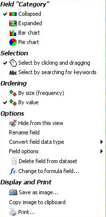 | Field "current field"- 4 options for displaying the field device: |
Note: The preview barometer count in the Text device may differ from the count in the Main Toolbar Barometer because the Text device barometer shows only the hits IN THAT FIELD, while the Main Toolbar Barometer shows the combined result of all selections across all devices.
Options, Display and Print- these commands are common to all views and documented in the sections on Data > Manage Fields [31] and View Tools [32].
![]()
| All charts- displays a list of all fields (columns) visible in the Chart View, with the same menu as the device right-click menu (see above) |
The rest of the commands shown above are common to all View Tools menus and are documented here [32]
Fields- used to choose which devices will be visible (ticked) or hidden (unticked). Also used to set the display order from top to bottom. Untick any fields you want to hide (you can bring them back later). Using the hands at the right of the menu, drag the fields in the menu upwards and downwards until you have them in the desired display order.
Collapse All- The Collapse All button on the Chart View Toolbar returns all expanded devices to their collapsed state. Clicking the small drop-down arrow next to Collapse all accesses a menu from which you can choose Expand All, Bar Charts or Analysis display modes.
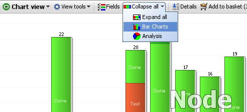
These menu items expand all the Chart View devices to one of their four possible display modes. For Number fields, Bar Chart mode creates a histogram for numerical fields with bands of values displayed both horizontally and vertically. Analysis mode shows a larger version of the plotted curve as well as key statistics on the numerical distribution. These statistics naturally update every time a query is executed. For Category fields, Bar Chart mode shows just that, while Analysis mode shows all the Category fields as pie charts. Selections of records can be made from all display modes directly with the mouse. Text fields do not display differently in Bar or Analysis display modes.
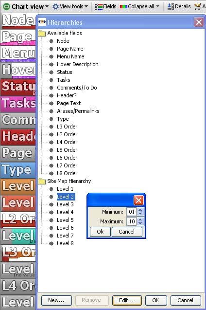
Categories which naturally 'nest' inside others, like Regions, Countries and Cities, can be combined in a hierarchy called, for example "Location". If records from more than one Region are in the IN Universe, the Chart View will display the Regionals in a new device called Location. Once only a single Region is selected, the Location Bar will 'drill down' and show the Countries in that region. If only one country is selected, Location will show only the cities in that country.
Creating a new hierarchy is easy...just give it a name, "Site Map Hierarchy" in the example below...then drag the fields (columns) comprising the hierarchy underneath in the order they belong.
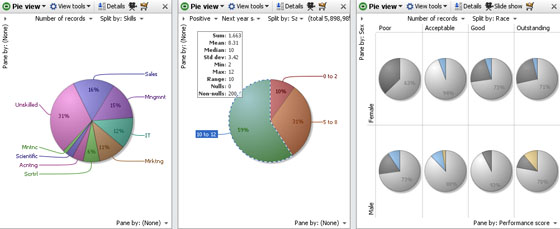
The Pie View shows a proportional breakdown of your data, either categories, or numeric. The default on opening for the first time is to show the breakdown by number of records. You can select the field to display and the field to use to split the pie into segments by using the view controls. If your data set has both positive and negative values, you can specify which to plot. You cannot plot both positive and negative values on the same pie, but you can use two Pie Views side-by-side for this purpose. If you must show both positive and negative values in relation to each other, use the Bar View [33].
You can select subsets of the data set on the pies, then execute ![]() Moves and
Moves and ![]() Keeps. You can also pane the Pie View vertically, horizontally, or both to obtain multi-pie views, as shown at right in the example below.
Keeps. You can also pane the Pie View vertically, horizontally, or both to obtain multi-pie views, as shown at right in the example below.
Field selector- shows all the fields whose values can be divided into segments. The default is to display the number of records divided by the field chosen in the adjacent Split-by drop down. You can choose a text field (column) to display, but if you do, the breakdown will be by number of characters in the text string values.
Split by- click on the ‘Split by’ drop down to choose a field to use to create segments within the pie(s).
Pane by- paning means displaying more than one pie chart within the display, horizontally, vertically, or both as shown in the example above right. Pane by field (column) selectors in the upper left and lower right of the Pie View display enable you to select criteria for generating multiple pies within the same Pie View. This is not the same as using two different Pie View windows.
When paning, you can use the 100% panes option in the View tools menu (see below) so that each of the multiple pies shows a breakdown totalling 100%. Use paning sparingly...if there is not enough space around each pie, Omniscope will not be able to display the labels, as shown in the example above.
The View tools drop-down menu offers a number of options
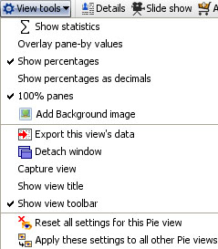 | Show statistics- when ticked, displays a translucent statistics panel, the content of which can be configured using a side menu accessed from the top of the panel. (see below) |
Add background image- provides the option to provide a faded image as a backdrop. See Page Menu [34] for details.
The rest of the commands on the View tools menu are common to all views and are documented in the section on View Tools [32]
The statistics panel display can be configured using the drop-down menu accessed from the upper right corner of the panel.
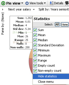 | 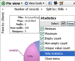 |
If the field (column) displayed is numeric, there will be more types of statistics available. If the field is a category field, summations, means, etc. will not be available.
Right-clicking anywhere on the Pie View window displays a menu of options to modify or export the display:
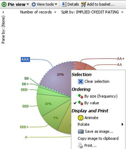 | Selection options: Ordering options: Display options: |
Copy and Print options:
Save as image or Copy image to clipboard- saves or pastes an image of the Pie View display (.JPG, .GIF, .PNG or .BMP depending on Java version) into another document.
Print- launches the Print wizard common to all views and documented in View Tools [32]
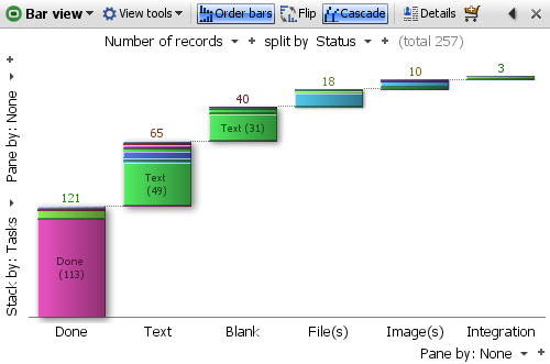
The Bar View is one of the most flexible views. It can be used to display either Category, Date and Time or Numeric data and calculated values like sums and averages. Both positive and negative numeric data can be compared in the same view. Bars can be displayed vertically or horizontally, and you can configure one or more splits (breakdowns) of selected values, with sub-breakdowns within the bars (stacked bars) and paning to create multiple displays in a single window.
All segments displayed in the Bar View are selectable, and can be used for power queries using the ![]() Move and
Move and ![]() Keep commands located on the Main Tool Bar.
Keep commands located on the Main Tool Bar.
In addition to the View Chooser and the View Tools drop-down menu, the View Toolbar contains a series of options for modifying how the bars display; Order bars, Flip, Cascade, 100% bars, Normalise panes, and Swap panes, plus the Show details, Slide show and Add to Basket commands common to all views and documented under View Toolbar commands [32].
![]()
View Tools- in the Bar View, all the view-specific commands are located on an Options pull-out menu accessible from this menu, and also accessible from the < arrow on the View Toolbar just left of the [X] close view command. All View Tools commands in the Bar View other than the link to Options (see below) are common to all other views and documented here. [32]
Order bars- sorts the bars in order of the values displayed, clicking again reverses the sort order, and again removes the sort.
Flip- changes the layout between horizontal and vertical bars
Cascade- displays the bars on a rising, progressive 'stair-step' base, rather than a single level.
100% Bars- normalises the height of each bar so that proportional differences in the stacked sub-segments inside each bar can be compared across the bars.
Normalise panes- normalises the height of the tallest bars in each pane, so that big differences in the absolute numbers do not minimise the height of the bars in some panes.
Swap panes- changes between horizontal and vertical paning.
See the Options sections below for more detail on the configuration options available.
Controls within the Bar View are located around the edges of the view. The Value and Split by menus are at the top, with Stack by and vertical Pane-by commands along the left side, and horizontal Pane-by menu at the bottom. Bar View configuration options are so numerous they have been put on a series of 6 drop-down menus accessed from a pull-out Options tab that appears whenever you hover your mouse along the right side of the display window.
Value/+ Add field Selector- left-most above the display, this drop-down menu allows you to select the quantity to be represented in bars. The default is the number of records, but you can change or add to the value field(s) being shown from this drop-down menu. You can toggle the field pick list to show all fields, numeric fields only or date fields only. Clicking on the '+' after the selector allows you to add another field as a quantity to display as an additional, separate bar next to the bar representing the first quantity. If you want to show the composition of each bar using the Stack-by option menu at left, you may want to select the 100% option to normalise the height of all the bars such that the stacked segments show comparable proportions. You can also specify the fields/values to represent on the Options > Measures menu (see below), which also offers additional sub-menus to specify the function being applied (sum, mean, standard deviation, etc.).
Split by/+Field Selector- drop-down menu allows you to specify one or more category, numeric, date or text fields to define how to break down the fields being plotted. You can also specify one or more fields to break down the values displayed using the Options > Breakdown menu (see below). Note:Split by selections are applied before Pane by selections.
Stack by Field Selector- (left side)- specifies the field to be displayed inside of each bar to create a 'stacked' bar chart. You can also access this command using the Options > Breakdown menu (see below).
Pane by/+ Add another Selectors- (left side & bottom)- paning creates separate sub-windows within a single display, which can be used to further break down the bars being displayed. You can also access these commands from the Options > Paning menu (see below). Note: Pane by selections are applied after Split by selections.
The Options tab menu contains 6 sub-menus; Measures, Breakdown, Paning, Ordering & alignment, Layout and Style.
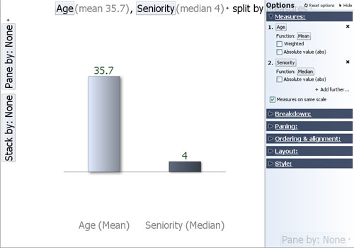
The Measures sub-menu is used to specify the values to represent as bars. In the example below, the Age and Seniority of employees is being plotted. Both of these are Numeric fields measured in the same units, years, so we use the Function sub-menu to specify that we want to plot the Mean (average) of the Ages and the median (most common value) for Seniority.
Value+ Add further fields- same as the field selector at the top left of the view, the Options dialog offers more options to specify functions, etc.
Function- only visible if you select numeric value fields (other than the Record count default). In the example above, the functions sub-menu is used to select average for the Ages (the sum would not be meaningful). The mean (average) age of the workers will not be weighted by the values in another field, so the Weighted option is not ticked. For the Seniority field, the median value, rather than the mean, will be displayed. There are no negative numbers in the Age or Seniority fields, so we will not need the Absolute value function either.
Measures on the same scale- since both values being plotted are in comparable units (years), we tick this option.
The Breakdown sub-menu allows you to plot additional bars by splitting the display according to other fields (columns) in the data set. In the example below, we split the display of average age and median seniority of employees by location.
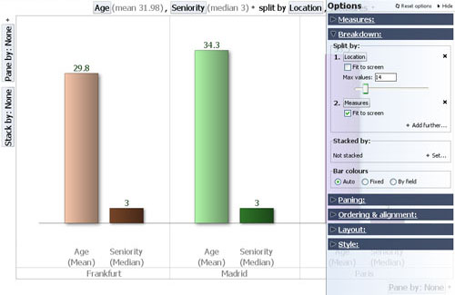
Split by: same as the field selector at the top of the display, the Options dialog offers additional options to control how the increased number of bars is displayed. If you choose a Split-by field with numerous values, you are also given a choice of displaying a bar for each value, grouping the splits into ranges (histogram), or grouping the bars by sign (positive or negative).
+Add further splits... allows you to specify further fields to sub-divide the bars by
Fit to screen- tick this option if you want all bars to display in the view window, no matter how compressed the width of the bars.
Max values- use this slider to manage the number of bars displayed individually. If the total number of bars is more than the viewable maximum, the remainder of the bars will be shown aggregated into an 'Others' grouping. The 'Others' grouping will be disaggregated only if filtering reduces the number of bars to be displayed to less than the maximum.
Stacked by: same as the field selector on the left, you can select only one field to display inside the bars, and you cannot mix positive and negative values.
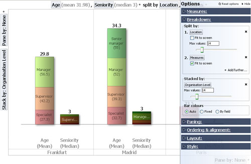
Max values- use this slider to manage the number of stacked segments displayed individually. If the total number of stacked segments is more than the viewable maximum, the remainder of the segments will be shown aggregated into an 'Others' grouping. The 'Others' grouping will be disaggregated only if filtering reduces the number of stacked segments to be displayed to less than the maximum.
Bar colours- use these options to control the colouring of the bars and bar segments.
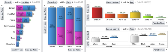
The Paning sub-menu is used to further sub-divide the display vertically, horizontally, or both. Paning sub-divisions are applied after Split-by selections. In the example below, the view display has been paned vertically based on the values in the Union membership field (column), which contains the values 'Yes' or 'No' for each employee. The resulting bar chart display indicates that Union members in this organisation are on average younger and most commonly less senior than non-union members, in both locations, London and Madrid.
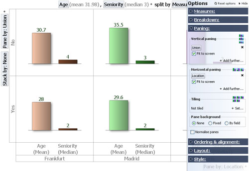
Vertical paning- same as the selector on left of display window, however the Options dialog offers more controls over how many panes to display unaggregated y if the number of values to panes by is large relative to the space available. To see all panes unaggregated, tick Fit to screen.
Horizontal paning- same as the selector on the bottom of display window, however the Options dialog offers more controls over how many panes to display unaggregated. Notice in the example above that the Split-by: 'Location' choice has been replaced by a horizontal Pane-by: 'Location' setting (faintly visible under the Options dialog panel at lower right). To see all panes unaggregated, tick Fit to screen. Note: Pane-by selections are applied after Split-by selections.
Tiling- adds multiple plots within each pane, showing the values further sub-divided. In the example below, we have left the display paned horizontally by 'Location' (values= Frankfurt, Madrid, etc.) and vertically by 'Union Membership' (values= 'Yes' and 'No'), and added Tiling by Sex (values: 'Male' in light and dark blue and 'Female' in light and dark pink):
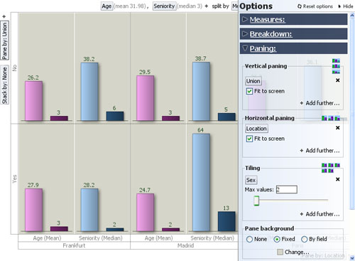
Note: Split-by and Pane-by choices are applied before Tiling. To see the values represented by the bars in each sub-plot (cluster) within the panes, hover on the bar with your mouse and the values are displayed in the Tooltip.
Pane background- use this command to set the background colour of the panes, which can be all the same or different.
Normalise panes- typically used in conjunction with stacking, sets the height of the (first) bars in all panes to be the same, regardless of their relative magnitudes, so that the proportions of the sub-segments representing the Stack-by values will be comparable across panes.
The Ordering & alignment sub-menu allows you to control the relative positioning of bars both within and across panes. The example below has the same settings as the one above, except that Order bar and Order vertical panes options are ticked, and the ordering is now set to 'Ascending'. Notice that in example below, the bars representing median seniority and average age have now changed positions, and that the Union='Yes' panes are now on top of the Union='No' panes:
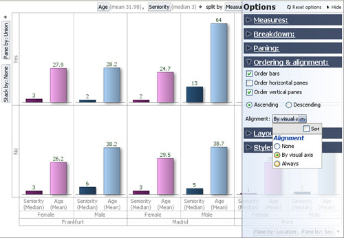
Order bars- sorts the bars within panes/tiles in either Ascending or Descending order. In the example above, the bars are in comparable Years units and the lower value, median Seniority, is displayed before the higher value, average Age. Changing the sort order to Descending will reverse the order of the bars within the panes/tiles. Behaviour of this option can be influenced by the Alignment settings (see Alignment below).
Order stacks- whenever a Stack-by field is specified ('None' is specified in the example above), ticking this option will sort the sub-segments within each bar in either ascending or descending order.
Order horizontal panes- when ticked, this option will order the panes horizontally, Ascending or Descending, based on the ranking of the values. In the example above, this option is not ticked. Behaviour of this option can be influenced by the Alignment settings (see Alignment below).
Order vertical panes- when ticked, this option will order the panes vertically, Ascending or Descending, based on the ranking of the values. In the example above, this option is ticked, and the Union='Yes' vertical panes are displayed above the Union='No' vertical panes. Behaviour of this option can be influenced by the Alignment settings (see Alignment below).
Alignment: comparison of bars across panes is facilitated by keeping the bars in a consistent order, especially looking vertically for a vertical bar orientation and looking horizontally for a horizontal bar orientation (see Options > Layout > Bar orientation below).
The Layout sub-menu is used to manage the appearance of each Bar View display. Most of the visual aspects , such as orientation, width and spacing of the bars, etc. can be managed from this dialog. In the example below, we have changed the bar orientation to horizontal, increased the minimum bar width and reduced the bar spacing to slightly overlap the bars:
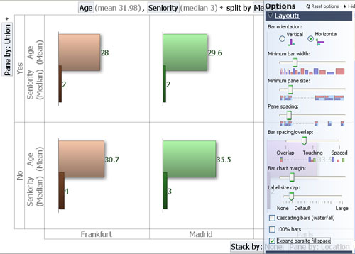
Bar orientation- changes the bars between vertical and horizontal directionality. Note that in vertical orientation, the Stack-by field selector moves from the left side to the bottom of the display
Minimum bar width- changes the minimum width of each bar in order to display more or fewer bars
Minimum pane size- changes the minimum width/height of panes in order to display more or less panes
Pane spacing- changes pane margin/spacing allocating more or less space in the pane to the bars.
Cluster spacing- {being revised}
Bar spacing/overlap- changes the space between the bars, which can overlap (see above), touch or be spaced apart
Bar chart margin- changes the margin space around the outer edges of the display
Axis label size cap- sets the maximum length of the labels, which can cause them to wrap or display vertically to save space. Warning: Setting Axix label size cap to 'None' (meaning no label) will suppress labels display completely. Start with the Axis label size cap set to 'Large' and reduce...working in conjunction with Style/Font Size (see below).
Measure/Axis font size - Allows you to control the font size of the measure labels and of those that are shown on the x or y axis.
Measure label orientation - Allows you to control how measure labels are shown (auto/vertical/horizontal). By default this is set to auto which means that bar view automatically calculates what is the best orientation of measure labels i.e. if there is not enough space to show all the labels horizontally fully then it will show them vertically. However, the auto behaviour may not be always be accurate in all situations in which case you can manually set the orientation.
Measure label spacing - Allows you to control how much space is allocated to measure labels when they are displayed. This option is particulary useful when measure labels orientation is vertical and you have big values, and you want to show the full value and don't want to truncation of the values to take place.
Cascading bars (waterfall)- same as the option on the Toolbar, displays the bars on a rising, progressive 'stair-step' base, rather than a single level.
100% Bars- same as the option on the Toolbar, normalises the height of each bar so that proportional differences in the stacked sub-segments inside each bar are comparable across the bars.
Expand bars to fill space- sets the bar widths so as to use all available space after allowing for settings governing margins, spacings, maximum bars and panes to show disaggregated, etc.
The Style sub-menu allows you control the visual effects applied to the individual bars. In general, we suggest that you use the default effects for best visualisation. Turning off the defaults will display the bars with no visual effects:
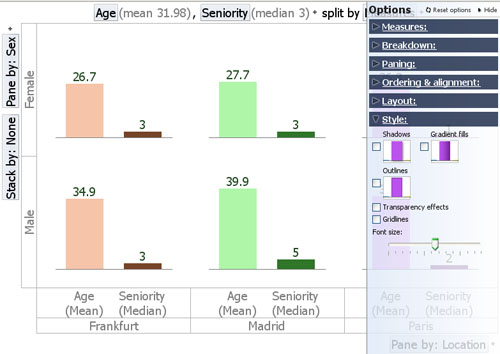
Shadows- adds a shadow effect to the side of each bar
Gradient fills- varies the colouring of each bar to give the impression of a more solid, reflective surface
Outlines- draws a solid border around each bar
Transparency effects- {being revised}
Gridlines- unticking this option will remove the border lines between panes
Font size- allows you to increase or decrease the label font size for best legibility
The Pivot View is used to display aggregated or summarised values at the intersections of fields (columns) in your datasets. Only Category fields are available on the drop-down menus, so if you want to create a pivot on a Text field, you should first either convert it (or a duplicate) to a Category field, assuming there are not too many discrete values. See Data > Manage Fields [35]for more detail on changing data typing and limits on the number of Category values.
Note: Pivot Views using Dates and Times and Numeric columns may be supported in future.
When you open a Pivot View and define two Category columns, Omniscope creates a pivot ( intersection grid of summary values) using the Sum of the number of records in two Category fields by default. You can easily change the Category fields to be displayed on the horizontal (X:) and vertical (Y:) axes using the View Toolbar options. At any time, you can exchange the( X:) and (Y:) axes by clicking on the curved arrow at the corner to the left of the horizontal titles.
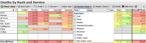
Value: the default value for the cells in the Pivot View is the sum of the records, so each cell will display the number of data points. You can change the value displayed to another field using the Value: drop-down menu. Depending on the type of field you select, a Function: menu will appear, allowing you to chose whether to display the sum, the mean, or some other transformation of the data points in each cell. Note: the Range function displays the difference between the maximum and minimum values in the cell. The example above shows the average age of military casualties by service branch and rank. If you choose a function such as mean, a Weight: menu will appear, allowing you to specify another field to calculate weighted averages of the values in each cell.
You can select one or more cells to perform ![]() Moves and
Moves and ![]() Keeps, but only on selections of all cells in one row or column at a time. You can sort the rows and the columns simultaneously; click the row or column header once to sort descending and again to sort ascending. The sorted column and/or row headers will turn orange to indicate sort(s) have been set. Clear your sorts using the [X] button that appears to the left of the switch axes curved arrow when sorts are set.
Keeps, but only on selections of all cells in one row or column at a time. You can sort the rows and the columns simultaneously; click the row or column header once to sort descending and again to sort ascending. The sorted column and/or row headers will turn orange to indicate sort(s) have been set. Clear your sorts using the [X] button that appears to the left of the switch axes curved arrow when sorts are set.
The Pivot View tools drop-down menu provides some options to change the display.
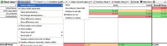
Colour relative to -
None- removes all coloring from cells
According to value field- applies the colouring range specified for the Value field (column) to display in the cells. The colouring range settings (start, middle, end, etc). are those defined for the Value: field in Data > Manage Fields > Configure > Field Options > Change Value colouring. This option will apply the absolute colors for the entire range of values, so applying it to calculated means and medians will not result in enough colour dispersion across the cells.
Relative to all cells- this option applies the colour range specified for the Value: field relative to the range of values appearing in the cells. Use this option to maximise dispersion of colours across reduced value ranges in all cells, typical of means and medians for example.
Relative to row- this option applies the Value: field colour range relative to the values in each row
Relative to column- this option applies the Value: field colour range relative to the values in each column
Colour totals separately- unticking this option changes the colouring scheme to include Overall totals columns values.
Value decimal places- use slider to set the number of decimal places to display fro absolute values
Percentage decimal places- use slider to set number of decimal places displayed for percentage values
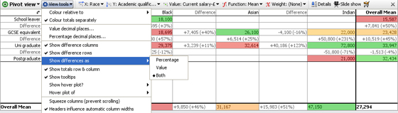
Show difference columns- when ticked, displays the differences between adjacent columns in a separate column (see below)
Show difference rows- when ticked, displays the differences between adjacent rows in a separate row
Show totals row - untick this option to hide the totals row that is shown at the bottom of the view.
Show totals column - untick this option to hide the totals column that is shown the right hand side of the view.
Show difference as - ( Percentage; Value; or Both) - allows you to select how the values in difference columns and rows are displayed
Show tooltips - temporary displays of record counts and other underlying cell information on mouse hover can be hidden by unticking this option. Note: Pivot Table tooltips are summaries of the values underlying each cell, not the record-level tooltips configured under Main Toolbar > Settings > Tooltips.
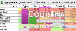
Show hover plot - ( None; Bar; or Pie) - a temporary graphical breakdown of the contents of a cell can be configured, either a Pie or a Bar chart display.
Hover plot of - (field list-Category & Numeric data types) - if a graphical cell hover display is selected, an additional option to specify the value to be plotted appears. In the example below, a Bar chart plotting the field Country has been configured. Hovering on the intersection cell Service:Army & Rank:Corporal, displays a Bar Chart of Countries losing one or more Army Corporals (average age: 24.13 years) plotted as vertical bars in descending order:
Squeeze columns (prevent scrolling) - keeps the column widths set to a distance that permits all columns to be seen/selected without horizontal scrolling of the view. Combined with row and column colouring options, this can convert the Pivot Table into a type of 'heat map' encompassing a large number of cells at a glance.
Headers influence automatic column widths - when ticked, re-sizing one column header re-sizes all of the other column headers to match.
The remaining commands on the View tools drop-down are common to all views and are documented here [32].
The Graph View (or scatter plot) is ideal for finding and illustrating relationships in the data. In addition to plotting two selected fields (columns) on the familiar orthogonal Cartesian axes, X (horizontal) and Y (vertical), you can colour, size and shape the markers to represent multiple dimensions in the data set. Markers can be clustered to group data points for large data sets, or displaced slightly to make coincident points distinct and selectable. Powerful statistical analysis is available, and various selection and display modes can be chosen to suit any combination of fields plotted.
Axis Selectors (X and Y)- use these pick list menus on the left side and bottom of the window to choose appropriate fields (columns) to plot on the X and Y axes. Only numeric, date and category fields will be present in the pick list. Text fields cannot be plotted unless the values are converted to categories and ideally given a meaningful sort order using Data > Manage Fields. Use the Sort option to sort the available fields alphabetically and the Find/Clear tool to select from long field lists. Note: hiding fields (columns) from the axis selector lists is not currently supported.
Switch Axes- the double arrow at the lower left of the plot exchanges the X and Y fieldsThe Graph View Toolbar features a View Tools drop-down menu, plus Trends, Mode, Zoom, Colour, Size and Shape options:
![]()
Each of these Graph View Toolbar elements is discussed below
The Graph View > View Tools drop-down menu includes various options for changing the display:
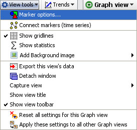 | Marker options- see discussion of sub-menu below Add background image-click to browse to an image to set as a faded background for the graph. Does not obscure gridlines. Useful for putting logos and branding into the display. The same option is available in the Pie, Bar and Details View and is fully documented here. [34] |
The other Graph View > View Tools commands are common to all views and fully documented here. [32]
Marker Options- click to launch the Marker options sub-menu, which has both Simple and Advanced display modes:
Marker Options: Heat Map, Clustered or Displaced- tick one to select from 3 different ways of displaying plotted points in each Graph View:
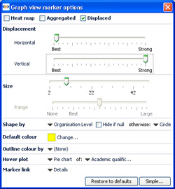 | Heat Map- shows density plot of records on the grid. Useful for plotting very large numbers of records that overlap a great deal. |
Displacement- changes the amount of displacement vertically and horizontally to improve access to data points for selection and linking.
Size slider- changes the absolute scale for marker sizing to increase or decrease all marker sizes
Range slider- (greyed-out unless the Size option is set to a field) changes the magnitude of relative sizing (see Size below)
Shape by: selects the field (column) whose values will determine the shapes plotted (same as Shape: toolbar pick list below) with additional options to specify the display of markers of records which are null (blank, not zero) in the selected Shape by field. In Simple mode, the Default shape to use when no Shape-by field has been chosen can be set.
Default colour- selects the default colour of markers when no other colouring options are set.
Outline colour by: adds an outline of another colour, based on another filed. For example, if Sex is used, this command would put a blue outline on the dots representing males and a pink outline on the dots representing females- assuming that you have assigned the those colours to the values 'Male' and Female'.
Hover plot- sets a pop-up display of either a pie or a bar chart whenever the user hovers on a marker, clustered or not. When set, you can select the field (column) to be charted using the pick list at right, which is otherwise greyed-out.
Marker link- selects a link to display when markers are clicked (one record only). Pick either (None), Details, or one of the links already configured in the file using the Settings > Links wizard accessed from the Main Toolbar.
Connect Markers (time series)- clicking this option expands the View Tools menu to display additional options used to configure connected series, usually time series. In order to display one or more time series curves, the data set should contain at least one field (column) for a date, and one or more columns for values that make up the time series. To display multiple curves in one graph, there should also be a category field (with relatively few unique values) containing the names of each curve to be drawn.
Note: if your time series data is not in 'vertical' Omniscope layout (with the repeated observations vertical in a column) but instead in a pivoted 'horizontal' table (dates as columns and one row for each curve's values), you can use the Data > De-pivot the data option on the Main Toolbar to change the layout. For more on how to lay out your data for display as time series, see Data Layout-Time Series [36].
Once your data layout is correct, to display the curves, switch the X axis to the date field, and the Y axis to the value you want to graph, then select Connect markers (time series)'. Warning: to see multiple lines, you must use the Show line for each... option and select a Category field that distinguishes the lines you want to separate. The additional time series sub-menu options allow you to show the markers along the curves, change the curve thickness, display the curve names, smooth the curves, etc. For more detail, see Displaying Time Series [37].
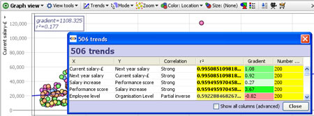
The Trends option menu enables you to access powerful statistical analysis of your data set, and to display the most significant relationships.
Clicking on this menu reveals two options:
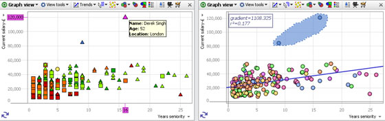
Show line of best fit-plots a blue line of regression 'best fit' through the data points with the R-squared (measure of correlation) and gradient values displayed in the top left corner.
Find trends-analyses and sorts all correlations and other advanced statistics across all columns in the data set. Click to calculate the first 100 best fits between all possible axes. These will show in a pop-up window with R-squared for each axis pairing. Clicking on a pairing in the window will load the corresponding graph into the view. Too see all standard calculations for all potential X/Y axis pairs. tick the Show all columns (advanced) option.
The Mode options menu enables you to choose how to navigate and select points and groups of points on the display. You can define one or more selection areas/shapes in order to exclude or isolate records using Move and Keep power query commands on the Main Toolbar. You can also use the mouse in navigational mode to define and explore specific zones in the display in maximum detail.
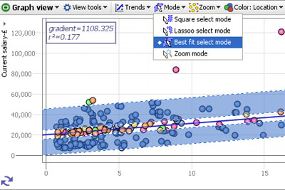
Square select mode- the mouse defines one or more rectangular selection area(s)
Lasso select mode- the mouse defines one or more free-form shaped selection area(s)
Best fit select mode- the mouse defines selection areas along the line of best fit. Useful for selecting data points inside/outside of confidence intervals in distributions.
Zoom mode- a navigational mode, the mouse defines a rectangular zone and the display zooms to show only that area. Holding the right mouse button down in zoom mode and moving the mouse up and down will zoom in and out continuously
Pan mode- (only visible when zoomed in manually) a navigational mode, the mouse 'hand' cursor is used to 'grab' the screen and move it to frame the desired area.
The Zoom options menu provides fine-grained control over the magnification of the display, and they way the display adapts to power queries and Side Bar filtering which change the distribution of the data points being displayed. Unless disabled (see below) when zooming, zoom bars will appear along the vertical and horizontal axes, which can be moved or stretched to display desired area on-screen.
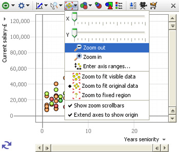
X zoom slider;Y zoom slider; Zoom out/in- used to expand the view along the right/left 'X' or up/down 'Y' axis, or to magnify (zoom in) or de-magnify (zoom out) the display.
The zooming options below are used to define how the display updates, with no manual zooming active
Zoom to fit visible data- display sizes to show only the points still in the target universe
Zoom to fit original data- display sizes to show the range of all the data in the data set
Zoom to fixed region- allows you to define a region of interest with the mouse, to which the display will revert, regardless of the data points in the target universe.
Note: the target universe for a given view is indicated by the colour of the view icon, green means IN universe, gold means BASKET, etc. For more detail, see Data Universes [38].
Show zoom scrollbars- when ticked, zoom scrollbars are visible even if the display is not zoomed, When unticked, the zoom scrollbars only show when zooming is active.
Warning: any manual navigation will take the display out of the default Zoom to fit visible data mode in favour of the Zoom to fixed region. You must manually change the setting in the Zoom menu to restore a default view of all the data in the target universe.
Extend axes to show origin- when ticked, the display is altered to make the 0,0 point where the axes cross visible in the display, regardless of the range of values in the fields (columns)
Enter axis ranges- used to define the range to be displayed numerically, based on the maxima and minima reported for the selected fields
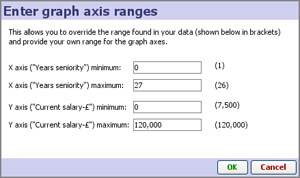
Depending on the size settings for the markers, you may need to 'pad' these ranges up or down somewhat to accommodate the marker sizing and achieve the optimal display.
The Size options pick list menu allows you to select the field used to calculate relative sizing of the markers in the display, regardless of the shape or the default size setting. The extent of the sizing effect is controlled by the Size and Range sliders available on the advanced Marker Options sub-menu.
When
clustering is active, where each marker represents more than one
record, you can choose the measure function (sum, mean, etc.) from the
bottom of the Size drop-down (2.5).
The Colour pick-list menu allows you to select the field to be used to colour the markers. If no colour is specified, a single uniform default colour is used (which can be changed (see above).
You can also use the application-wide Colour button on the main toolbar to enable colouring in all relevant views.
The Shape options pick list allows you to specify which field (if any) you would like to use to determine the shape of the marker to use on the plot. You can also set the Shape-by field in the Marker options sub-menu, as well as specify the treatment of null values in the plots.
If you configure colouring or shaping, the Key button appears, which will open a key showing the values and associated colours/shapes for that field (column).
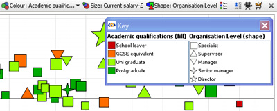
Note: At any time you can change the colours/shapes assigned to the values in a given field (column) using Data > Manage Fields > Configure > Field Options > Change value order, colours and shapes.
This section guides you through using the Connect markers (time series) options available in an expandable section of the View Tools menu of the Graph View (download the sample file used to illustrate this section here [40]).
Omniscope manages repeated observations of values over time in vertical columns, rather than horizontal rows often used for time series in spreadsheets. To create a multi-line time series as shown below, first put your data in the following 'vertical' orientation:
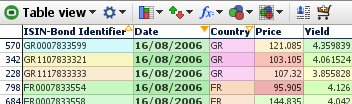
In the above example of a time series data layout for Omniscope, we have various bonds, each with an ISIN identifier, and each issued by one of various countries (GR, FR etc.). We also have repeated observations of Price and Yield over time entered vertically down the columns. Each record (row) in the data file is therefore a separate observation of price and yield which are repeated over time 'vertically' in separate rows
Time series data layout in Omniscope requires at least one field (column) with a natural order, such as Date, and one or more values columns 'Price', 'Yield', etc. for repeated observations of values that make up the time series. In addition, to display multiple curves on one graph, there should be a Category field (with less than about 200-250 unique values) referencing each curve to be drawn. In this example, we have many observations, but only 9 unique ISINs (individual bonds) so the curves can be plotted by the Category 'ISIN' reference field as shown in the example below. Don't worry about the apparent repetition in the data values, outside of the Table View, Omniscope will render the duplication invisible to you and the users of your files.
If your data is arranged differently from the example above, (e.g. 'horizontally' with the dates as columns and each cell in the row representing an observation over time) you may want to use the the tools available under Data > De-/Re-Pivot on the Main Toolbar to transform your data set to the correct 'vertical' orientation in Omniscope. More on Using De/Re-pivot [41].
Checking your data types: After importing and correcting the layout of your data, go to Data > Manage Fields [35] and make sure the Time (here Date) and Observation (here Price, Yield etc.) fields (columns) have the correct data typing. They must be typed Numeric (decimal or integer), or Dates & Times. Also make sure that any fields you want to use to distinguish lines (here the ISIN Bond Identifier number) are declared of type Category. You can convert data types using the Data > Manage Fields dialog or by by right-clicking the column header in the Table View and choosing Tools > Convert field data type.
Once you are sure that your data layout and field (column) data typing is correct, add a Graph View and configure the axes:
You will see an un-connected scatter plot of markers representing your time series data points. In the View Tools drop-down menu, tick Connect markers (time series). A number of new options should appear on an expandable sub-menu below this command on the View Tools menu.
WARNING: This option will be unavailable if the Graph View has been configured with Displaced (randomly offset) markers. Open the Marker options dialog above on the View Tools menu and confirm that the Displaced option is not ticked.
At this point, the display will change from unconnected scatter to connected plot, but with many heavy black lines in a jumble. The expanded sub-menu includes a number of commands used to manage the display of connected markers:
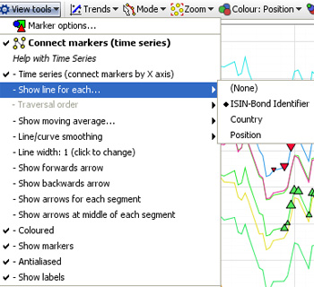
Time series (connect markers by X axis)- when ticked, automatically uses the field (column) selected for the X horizontal axis( here Date) to provide the traversal order, the order in which the dots are connected. This is the most common setting for time series. When this option is ticked, the Traversal order option below is greyed-out.
Traversal Order (showing an omni-directional path) By unticking Time series (connect markers by X axis), you can choose to draw the lines in a different order than dictated by the X axis. If you are plotting data based on criteria other than time, configure the Traversal order field appropriately.
Show moving average: None; Simple & Exponential- If you have many data points in each time series, you may wish to try showing a moving average, by choosing Simple, Exponential or other data smoothing options on the sub-menu.
Line/curve smoothing- By default, lines are turned into curves while preserving data points. In other words, curves are drawn between the data points. Depending on your data, this may be inappropriate. You can disable this using the Line/curve smoothing sub-menu. Alternatively, a second form of curve smoothing is provided, which does not pass through the data points. Untick Curves pass through vertex points to use this option. Both forms of smoothing can be adjusted for amount of smoothing using the Smoothing amount option.
Line width-By default, lines are shown 2 pixels thick. Use the slider to change this any value between 1 and 25 pixels.
Arrows: Show forward arrow; backward arrow; arrows for each segment; middle of each segment-adds different kinds of directional arrow heads to the line segments displayed
Coloured- By default, if you have multiple lines displayed, these are coloured according to the values in the Category field. You can disable this and show only black lines by deselecting this option.
Show markers- Hides or reveals the markers within the plotted lines (to resize markers, see Marker Options on the View Tools menu
Anti-aliased- Smooths the way the line is displayed
Show labels- By default, text labels will be shown beside each line if you have multiple lines. By de-selecting Show labels, these will only be shown as you move the mouse pointer over a line.
When Connect markers (time series) is enabled and lines are showing, the Line select mode becomes available from the Modes drop-down. Select this mode, and the mouse pointer will change to show that you are in Line select mode. Move the mouse pointer over a line, and it will become highlighted.
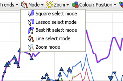
There are two ways to select records in Line select mode:
If you have made too many configuration changes and can't figure out how to get back, you can reset all settings for the current Graph View, returning to a plain default view with no marker connection settings enabled. From the bottom of the View Tools menu, choose Reset all settings for this Graph view.
The Tile View represents each record in the data set as a rectangular tile, which can be grouped, sized, sorted and coloured to display relationships, anomalies and outliers in the data. Tiles can be either image tiles displaying images associated with each record, or solid tiles displaying text and coloured and sized to represent various attributes of each record. The Tile View can be used as an image browser (see Open Image Set [42]), but it is also a powerful 'heatmap' (treemap) for representing data visually along multiple dimensions. Moving the mouse over the tiles reveals the title for the record. By default, clicking on the tile selects the corresponding record. Double-clicking on the tile brings up the details display.
The example below shows two Tile Views displaying the same collection of shoes. The Tile View on top is set to display an associated image set (the shoe pictures) as tile contents. Note the vertical scroll bar on the right, as the pictures have been up-sized from the default so that not all will display in the open view. The second Tile View below is showing the same collection of shoes using solid tiles coloured to match the colour of of each pair of shoes and sized in relation to price:
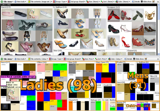
The Tile View is controlled using six configuration options located across the View Toolbar:
Tile Contents: this drop-down menu provides the option to display either data values as solid, text containing tiles, or associated image sets as picture tiles. If you select a data field, the value of that field will display inside the tile representing each record. If you select an image set, it will display the name of the image file on tile select/hover unless you change the ungrouped tile title to the contents of another field (see below).
Group: arranges the tiles into groups by any field. In the example above, the shoes are grouped first by Type: Ladies, Mens and Children's.
2nd Group: within the first grouping, arranges the tiles into sub-groups by the value in the specified field. In the example above, shoes are grouped secondarily by Brand/Designer.
Size: varies the size of each tile in proportion to the value in the specified field. Can be used with both image and solid tiles. In the example above, the solid colour tiles are sized in proportion to Price.
Sort: Sorts the tiles vertically by another field, such as Price.
Colour: determines which field value is used to colour the tile, and can be used with image tiles as a semi-transparent overlay. In the example above, Omniscope recognised and automatically applied the colours to match the all the values in the Shoe Colour field, except for cream, which was set manually. For more on assigning colours to specific values in a given field, see Data > Manage Fields [35].
The Tile View Tools drop-down menu contains several options to change the display and selection behaviour in the view.
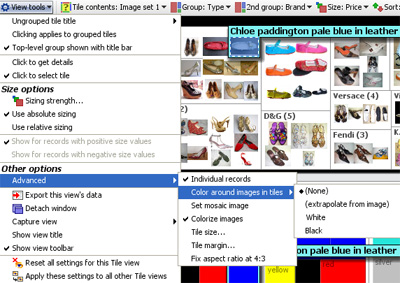
Ungrouped tile title- use this option to specify the value to be displayed on hover/selection instead of the value associated with the tile contents display value. In the example above, the Description text is showing, rather than the file name of the associated image file, which is sometimes not informative.
Clicking applies to grouped tiles- when ticked, this option enables you to select entire groupings, rather than individual tiles.
Top-level group shown with title bar- when ticked, this option displays the field by which the top-level grouping is defined as a nested title as shown in the examples above. When unticked, the title of the primary grouping field is displayed as a large orange text overlay on top of the primary grouped tiles, as shown in the lower Tile View example above.
Click to get details- when ticked, a single left click displays the details window for that record
Click to select tile- when ticked, a single left click selects that record
Sizing strength- this option is used to tune the sizing on a scale of -100% through 0 to +100%. The default is 100%, which means that the sizing calculation uses the default. Lowering the value to 0 eliminates all sizing, and further reducing it to -100% inverts the sizing, so that lower values get larger sizing.
Use absolute sizing- this option calculates the sizing of all tiles based on the entire dataset, and keeps them sized this way regardless of the sub-set of records in the open view.
Use relative sizing- this option re-calculates the sizing of the tiles based only on the records in the open view. Use this setting to accentuate small differences and counter the tendency of increasingly similar records to be sized similarly as the range of interest narrows.
Show for records with positive/negative values- the Tile View can be used either with all positive values being displayed, or all negative values being displayed, but not both. Use two open Tile Views like the example above to show both positive and negative values, or use the Bar View.
Individual records- ticked by default, if the chosen tile contents field is a number or date, unticking this option will aggregate values into ranges and show the tiles for ranges, rather than the individual values per record.
Show image for first token only- if your file has a tokenised image set (multiple images per record), by defaul the Tile View will show only the first image associated with the record. Untick this option to show all the images associated with the record.
Colour around images in tiles- the relationship between the height and width (aspect ratio) of pictures inside image sets is often not uniform, or does not match the shape of the Tile View display. Omniscope creates blank spaces between the pictures to fill the gaps. This option controls the colour of the background fill; none, extrapolate from image (estimated from the colours on the edge of the pictures), black or white.
Set mosaic image- used to create an effect in which a large high-contrast picture is re-created using many smaller images related to records in the data set. Cannot be used with grouping, sizing or sorting enabled.
Colourise images- when ticked, allows semi-transparent colour overlays to cover the entire image tile. When unticked, only the border fill space is colourised according to the values of the files selected in Colour: on the View Toolbar
Tile size- used to over-ride the default tile sizing which tried to ensure that all tiles display in the open Tile View without scrolling. If you increase the tile size, scroll bars will be added to the view as required. Relative or absolute sizing options are not affected.
Use grid layout- only shows when sizing is not active. Changes the allocation of space within groupings to make tile size uniform within each group.
Tile margin- used to increase the amount of background space displayed around the edges of the tiles. Colour around images settings are not affected
Fix aspect ratio at 4:3- used to make image collections appear more uniform and minimise distortion of images with 4:3 aspect ratio.
Right-clicking on a tile brings up a detailed selection menu where you can specify exactly the records you seek, and change the settings for the view.
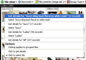
The commands available on the right-click menu under Options are the same as those available in the View Tools menu
The Network View creates a virtual network of interconnecting nodes in your machines' memory to help visualise relationships in your dataset. Each node within a network represents a data subset and lines connecting the nodes indicate the relationships between these subsets. You can use one of many inbuilt layout algorithms to position the nodes within the view, or use your mouse to move the node arrangement around to create a custom layout best suited to your data.
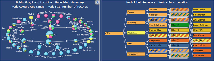
When you first open a new Network View you will be asked to select a network type. The network type determines how the network will be built based on the relationships in your data set. There can be more than one network type used for a given data set using multiple Network Views.
For any given Network View, there are two broad options for specifying the type of network you wish to visualise, Grouped Hierarchies and Relational Networks:
Grouped HierarchiesA grouped hierarchy can be used tovisualise almost any type of data. In a grouped network each node represents a group of records. Once you have selected a grouped hierarchy use the field selector on the Network View toolbar to definethe columns in your data set to be included within the network. Each field (column) chosen will define another 'level' within the hierarchy. At eachlevel, the records will be split by the associated field values. Relational NetworkArelational network can be used to represent any dataset where a commonrelationship exists between the rows. Each row should define a 'key' field and one or more 'linked fields'. The 'key' field should provide a unique identifier for the row entity. For example, for a data set comprised of people, the 'key' field might be the person's name, insurance number or other identifier unique to thatparticular person. The 'linked' fields create the linkage(s) to another entity, defining the key value for the linked entity, thereby allowing the network to determine which entities are connected. | 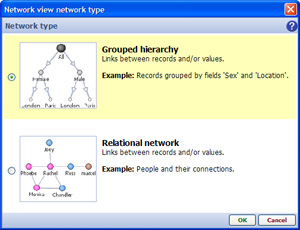 |
Like the View Toolbar displayed in other views, the Network View Toolbar contains a View Selector, Data Subset Selector and the Aggregate options drop-down menu that function in the same way as they do in other views. The View Tools drop-down contains first the commands specific to the Network View, and then the commands common to all views.
![]()
To the right of View Tools drop-down are the options menus specific to the Network View; Appearance options, Node options, Selection Mode options, Zoom options, Fields selector, Layout options, Navigator pop-up and Node Labelling, Colouring, Outlining and Sizing options. These menus are discussed in the sections below.
The Appearance options dialog [43] is immediately to the right of the View Tools drop-down. This is a large, multi-tabbed dialog that allows you to configure the colour, size and shape of the nodes, lines and labels within the network. There are three tabs; Nodes, Lines and Labels, with many options on each tab.
Nodes [44] - options relating to the shape, size, colour and images used to represent the Nodes in your data
Lines [45] - options relating to the display, thickness, colour, arrows and arrow positioning of the Lines between the Nodes
Labels [46] - options relating to the display of labels, field (column) names, empty values, and the spacing, alignment, fonts and background used
All of the Appearance dialog options on all three tabs are documented here [43]The Node Type options allows you to choose how nodes in the network will be portrayed. The Network View currently provides two node shape options: markers for which a range of shapes can be selected, and square/rectangular boxes.
| Marker - a marker consists of an arbitrary shape and a label shown adjacent to the marker. The marker option is particularly useful when visualising networks with a large number of nodes. |
This menu provides users the option to control the behavior of the mouse when navigating and filtering the network. The mouse mode options in the Network View are the same as those used in other views, such as the Graph and Map Views.
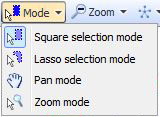 | Square selection - allows you to select and move node. To select one or more nodes hold down the left mouse button and drag the mouse across the view panel. A rectangular shape is created as a result of dragging the mouse. All of the nodes that are enclosed within the rectangular shape are included in the selection. To move a node simply move the mouse over the top of the node, hold down the left mouse button and drag the node to the desired location. You can move several nodes at once by selecting the nodes then moving any node from the selection. Lasso selection - lasso selection is used in the same way as the square selection; the difference is that a flexible lasso shape is used to manage the selection instead of a rectangle. With a lasso you can move the mouse to create a free-form shape, thereby allowing for more complex selections of one or more free-form areas. Pan - The pan mode allows you to navigate the network by moving the screen to frame the desired area. Once you select the pan mode a 'hand' icon will appear. Hold down the left mouse button and drag the mouse to move the window in the corresponding direction. Whilst using the pan mode you can use the mouse wheel to zoom in and out of the network. Zoom - The zoom mode allows you to zoom in or zoom out of the current network. To zoom to a specific area hold down the left mouse button and drag the mouse to create a rectangle highlighting the area to zoom to. To zoom in or out of the map hold down the right mouse button and drag the mouse up (to zoom in) or down (to zoom out). |
Zoom options in the Network View are very similar to those provided in the Graph and Map Views. The slider and the zoom buttons allow you to increase or decrease the magnification level. The following additional controls are provided:
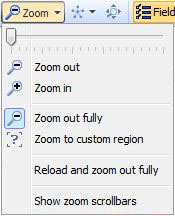 | Zoom out fully - Zooms the graph out to the full extent. This menu item is highlighted whenever the network is zoomed out fully. Zoom to custom region - Changes the interaction mode to the 'Zoom' mode. This menu item is highlighted whenever the network is zoomed to a custom magnification. Reload and zoom out fully - Reloads the entire graph, applies the current layout algorithm and zooms out to the full extent. Show zoom scrollbars - Indicates whether the zoom scrollbars are displayed. The zoom scrollbars are shown to the right and at the bottom of the view. They allow you to both zoom and pan the view window. |
The Fields chooser allows you to define which fileds (columns) are displayed or hidden, and functions just as it does in most other Omniscope Views
Specifying Layout Options allows you to apply a pre-defined layout algorithm to the current network. The position of the Nodes within the network is determined according to the parameters of the chosen layout algorithm. The Network View currently provides seven layout algorithms:
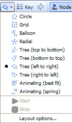 | For examples of each, see Layout Examples
|
Under the Layout selection drop-down is a link to the Layout options dialog, which allows you to modify the behaviour of the various layout algorithms.
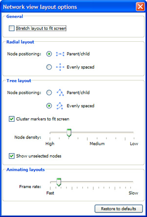 | General: Stretch layout to fit screen - If this optionis checked all of the nodes in the layout will be stretched out so thatthe maximum amount of screen space is used. Stretching is done bydefault in some layouts (Tree, Grid), and this preference will have noeffect if one of these layouts is in use. A good example of the effectchanging this preference can have is to create a network and select the'Circle' layout. Now select 'Stretch layout to fit screen'. You shouldsee the circle of nodes stretch out to form an ellipse. Radial layout: Node positioning - defines how the node position is determined when the radial layout is in use:
Cluster markers to fit screen - when checked, nodes too close together are 'clustered' tocreate a single node. Clustering can only be applied if the network ishierarchical, i.e. it has a root node, and the root has zero or more childnodes that in turn have zero or more child nodes...with each node having asingle parent node. Node density - determines how close nodes have to be to each other before they areclustered. If the density is set to 'High' then the space between eachnode is reduced, therefore allowing for a high number of nodes. If thedensity is set to 'Low' then the space between each node is increased,equating to a small number of nodes. Show unselected nodes - determines whether nodes which have not been selected are shown. Animating layouts: Frame rate -The Network View currently provides two animated layouts:Spring and Best fit. Use this slider to determine how fast thelayouts run. If your network is large and complex, setting a fast speedcould have a detrimental effect on performance. |
Click on the 'Navigator' button to open a small network navigation window. The navigator window will be docked on the right hand side of the view however it can be dragged and placed anywhere on screen.
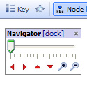 | Zoom slider - Moving the zoom slider or clicking on the Zoom In or Zoom out buttons allows you to increase or decrease the magnification. Navigation arrows - Clicking on the red navigation buttons allow you to shift the view in the corresponding direction Zoom magnifiers - |
Network View Toolbar - Node label
The Node Label drop-down allows you to determine how the label attached to each node is constructed.
The dropdown provides three types of measure:
|
Network View Toolbar - Node colour
The Node Colour drop-down menu allows you to specify the measure used to determine how Node colouring is calculated.
There are currently three types of measure:
|
Network View Toolbar - Node outline
The node outline drop-down menu allows you to specify the measure used to determine how the node outline is calculated. The Node outline option can be used in exactly the same way as the Node colour menu. You might find it easier to identify the node colour outline by increasing the outline thickness. You can modify the outline thickness using the Node options dialog.
The node size drop-down menu allows you to specify the measure used to determine the size of a node in relation to the other nodes on screen.
There are currently three types of measure:
|
The Network View Appearance options dialog has three tabs; Nodes, Lines and Labels
The Nodes tab contains options to configure almost all aspects of how Nodes are displayed, including display of images to represent Nodes.
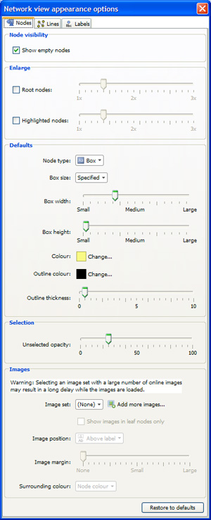 | Node Visibility: untick box to hide empty nodes in the display Enlarge: set the enlargement scales for both Root Nodes and Highlighted Nodes Defaults: Node type - choose either round 'Marker' or square 'Box' Marker options: (only shown when Node Type is set to 'Marker)
Colour - select the node background colour. Selection: Unselected opacityWhen you make a Selection within the Network View all of the selected Nodes appear blue whilst the unselected Nodes appear slightly faded.The unselected opacity slider allows you to define the fading level forunselected Node. A value of '0' means the nodes don't fade at allwhilst a value of '100' means the Node disappears when de-selected. Image set - Allows you to define an image set and display images from that set in the corresponding nodes on the network.
|
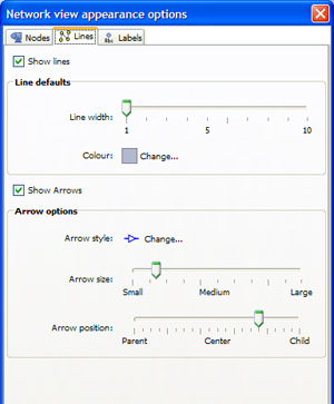 | Show lines -
|
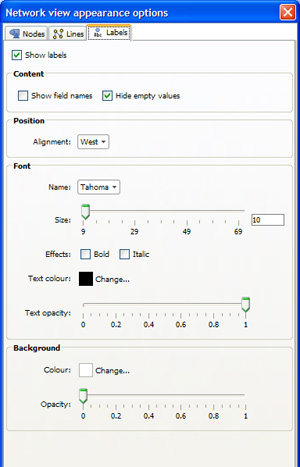 | Show labels -
|
The Portal View summarises most aspects of the data set (it can search but does not display text fields) as either field (column) value breakdowns (left example below), or statistics (right example below), or a mix of both. The optional search box works like a search engine across the entire data set, and the dynamically-generated range breakdowns can be selected for use in power queries using the Move, Keep and Reset commands.

The Portal View features a global Search Box used to select text string values from anywhere in the data set. This is equivalent to the 'Search all' filter device available on the Side Bars. Selection is done by typing into the keyword box (hits are shown in the preview counter on the far right as each character is typed. Multiple words can be entered and the 'and/or' relationship set using the 'ALL' and 'ANY' buttons to the right of the text search box ('ALL' is the default). Note: there is not currently an 'EXACT' option for use with numbers, etc.
The Search Box can be used in conjunction with the individual fields in the Portal View by entering text in the Search Box and selecting one or more value ranges within the view. The keyword 'hits' will be displayed in the Search Box while the overall number of hits (text and other values) will be shown by the blue preview bar inside the green barometer on the Main Toolbar. Note: the blue preview bar is only visible when selections are made. Any combination of text string input and multiple field range criteria can be selected and used to execute power queries using the Move and Keep commands on the Main Toolbar. The Search Box can also be used very effectively in conjunction with other views, such as the Table or Details Views set to display the SELECTION universe.
Field Settings menu- each numeric, date or category field displayed has a small black downward pointing arrow that reveals a Portal View filed display configuration menu with 3 options:
Show value breakdown- displays selectable dynamic ranges of the values in the field. Each field displays up to five categories, ranges, or intervals as a default. Additional categories are grouped into a category named ‘Other’. Numerical fields are broken into intervals necessary to make five groups of records. The fields containing collapsed categories are underlined. Click on any underlined field title to expand that field and see all categories or smaller numerical intervals. Click again to collapse it again.
Expand- expands the number of ranges displayed. If Show value breakdown is not selected, this option is greyed-out.
Show statistics- displays a pick list of statistics available for each field (column). Tick those you want to display, with or without the value ranges:
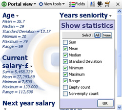
The Portal View tools drop-down menu features a number of options to configure the display. The Fields menu adjacent displays a pick and ordering list used to hide or show fields. Click and drag on the hands to change the order of the fields in the view.
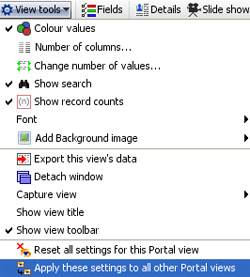 | Colour values- when ticked (the default), colours the values in line with other view colouring. Untick to remove colouring. Number of columns- changes the number of columns in which the field ranges are displayed. The default is two columns. Change number of values- changes how many categories or numerical ranges or intervals are shown under each field title when collapsed. The default is five categories/ranges (intervals) as shown above. Show search- shows or hides the global Search Box Show record counts- shows or hides the number of records per category or interval in each field. The default is to show the counts. Font- allows you to select font name, face and size (not colour). |
Add background image- enables you to add a faded image to the backdrop of the view. Same as the option provided in other views and documented in the Page Menu [47]commands.
The other options on the Portal View Toolbar, Show Details, Slide show and Add to Basket are common to all views and documented in the section on View Toolbar. [32]
The Map View is a powerful and flexible option for displaying spatial data at any level; world, country, city or even exhibition or office floor plans or sports playing fields. Omniscope embeds its own multi-layer vector maps that let you choose to display various geographic map layers (roads, mountains, sea depths, etc.). Omniscope comes with the world map shown below, but you can also download hundreds of other free country, regional and city maps from the Maps Library [48] for embedding in your Omniscope files.
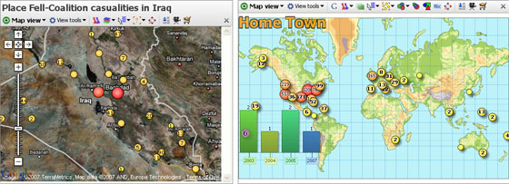
Using any activated edition of Omniscope, use the File > Open map > Download maps option to install and display new maps with blank data sets, which you can either ignore or start populating with your data. To load a scanned image or photograph for use as a backdrop, use the File > Open map > Browse for image or map file command.
Note: Omniscope currently imports Image (.JPG, .BMP, .GIF, .PNG depending on your Java version) plus Visokio's own .VEC, .MAP and .ILF file formats for use as coordinate backdrops in the Map View. If you save an .IOK file containing embedded image map(s), Omniscope will bundle them into the .IOK file so that anyone with the free Viewer will see the file with the correct map(s).
Each record (row) in your data sets can be associated with a marker displayed on the map, as long as the two designated map coordinate columns contain non-null, valid decimal coordinates. Using Place marker mode, you can add coordinates to your data set by opening a map view (or Google Maps), zooming in to show enough detail, then pointing at the location of each record with your mouse. More on Placing Markers [49]...
Details for each record are available by clicking on the marker representing the record or aggregated group of records. Note: if the Details view is not open, groups of four records or less will be displayed as a cascade of individual details windows, one per record, while markers aggregating five or more records will display the pop-up Show details table window showing the selected records with links to display individual details.
The Map View Toolbar includes the View Tools drop-down menu, an option to switch back and forth between vector and Google maps, a Map (Map Type for Google) selector, a Layer pick list, choice of mouse Mode and Zoom navigational controls, plus field (column) pick lists to set Colour, Sizing, Shape and Label options.
![]()
The Map View also features a pop-up Navigator overview mini-window, plus the Show Details, Slide Show, Add to Basket and [X] Close View options common to all views and documented here. [32]
Switch to Google/Vector Maps- to the right of the View Tools drop-down menu this option allows you to switch from the default vector map to a Google Map view which uses the same coordinate columns. When you are using Google Maps, this option label changes to Switch to Vector Map.
Suggestion: Placing, moving and correcting coordinates using the mouse in Place Marker Mode using Google Maps works well. However, if you are manually editing, deleting or cutting and pasting coordinate data with an open Google Maps display, make sure that the Zoom setting is NOT Zoom to fit visible data. If you are scrubbing and filtering data and find your Google Map display updating slowly or not displaying properly, switching to the corresponding vector map, then switching back will usually restore the display in Google Maps.
A tutorial on navigating in the Map View is available here. [50]
The Map selector is used to change the map in the view, or add a new vector map to the file. The drop-down menu shows the list of maps already configured in the file, with the currently displaying map ticked. Below that is the option to add another map from those already downloaded onto your machine, or by downloading additional maps from the Maps Library [48]. If you select to add a new, unconfigured map to the file, the Configure Map wizard will appear (see above) so that you can define a title and specify the coordinate fields (columns) to be used with the new map.
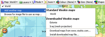
There is also an option to import your own map as an image in formats supported by your version of Java, plus Visokio Map formats (.VEC,.MAP,.ILF). Click on Browse for image file to use as a map, then browse to and select any image you choose. It will appear in the Map selector drop-down map listing menu as part of your growing collection. You can use any kind of photograph or scanned image as a Map View backdrop for placing data points. Typical examples include sporting fields, exhibition hall, office or factory floor plan layouts, banquet seating arrangements etc.
When displaying a Google Maps as a backdrop, the Map selector becomes Map Type, and allows you to chose from 3 options for the Google Map display: Map, Satellite and Hybrid:
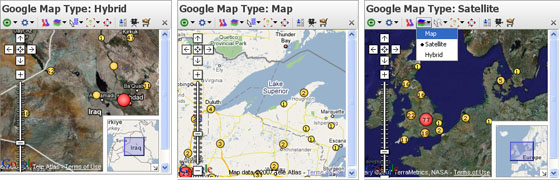
Choose one or more Google Map types that best suits the purpose of each display.
The default map is a Mercator projection world map with physical and political information in a series of configurable layers. With the default world map open, click ‘Layers’ to choose what to display. Click 'Physical' to hide or show physical altitudes and reveal the 'Political' layer. Tick or untick layers until you have the map you want.
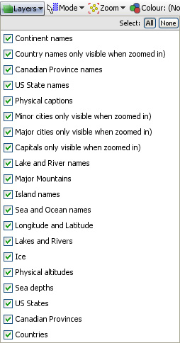
Note: some layers, such as capital, major and minor cities, will not be visible when zoomed out. Omniscope shows map detail progressively, only when the view is close enough to make sense of it. As you zoom in, more and more detail will appear, revealing the layers you have chosen.
If you would like to develop your own layers for distribution in .IOK files for display on vector or Google Maps, please contact us.. [51]
Map View selection Mode options are very similar to those used in the Graph View [52], including mouse-defined Square select and Lasso free-form selection as well as Zooming, and Panning navigational modes.
The Mode options menu enables you to choose how to navigate and select points and groups of points on the display. You can define one or more selection areas/shapes in order to exclude or isolate records using ![]() Move and
Move and ![]() Keep power query commands on the Main Toolbar. You can also use the mouse in navigational mode to define and explore specific zones in the display in maximum detail.
Keep power query commands on the Main Toolbar. You can also use the mouse in navigational mode to define and explore specific zones in the display in maximum detail.
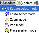 | Square select mode- the mouse defines one or more rectangular selection area(s) Lasso select mode- (not available in Google Maps) the mouse defines one or more free-form shaped selection area(s) Zoom mode- a navigational mode, the mouse defines a rectangular zone and the display zooms to show only that area. Holding the right mouse button down in zoom mode and moving the mouse up and down will zoom in and out continuously Pan mode- (only visible when zoomed in manually) a navigational mode, the mouse 'hand' cursor is used to 'grab' the screen and move it to frame the desired area. |
Place Marker mode- used to place markers for selected records, thereby generating values for the coordinate fields in the data. To do this, open a Table View and select a record with no coordinates/map marker by clicking the row header (or multiple records using the Shift or CTRL keys). Once selected. go to the open Map View, and with Mode set to Place marker mode, click on the point you want to locate the selected records on the map. In the case of the Visokio and Google world maps, the correct decimal longitude and latitude values will be placed in the coordinates columns. In the case of other maps, the coordinates will be relative to the specific map. For more detail, see Placing Markers [49].
The Map View Toolbar Zoom selector is also very similar to that used in the Graph View. The slider and Zoom out or Zoom in controls increase or reduce the magnification, changing the area and amount of detail/layers displayed.
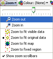 | Zoom to fit:
|
Show zoom scroll bars- when ticked, displays the zoom scroll bars bottom and sides at all times, even when zooming is not active.
Marker Colour, Size and Shape options are all defined with field pick lists available under each of these Toolbar options. If any of these options (or the Marker outline colour by option available in Marker options-see above) are set, the Key display also appears to help the reader relate the appearance of each marker to the underlying data.
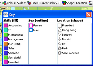
NOTE: You set the colour and shape associated with each different field (column) values using Data > Manage Fields available from the Main Toolbar. The intensity of the relative sizing effect is controlled with the Size and Range sliders in the Marker options Advanced menu (see above).
The Label drop-down selector enables you to choose the field to display next to all unaggregated markers. Aggregated markers show the label (mixed) until zooming or selection results in disaggregation to a single record.
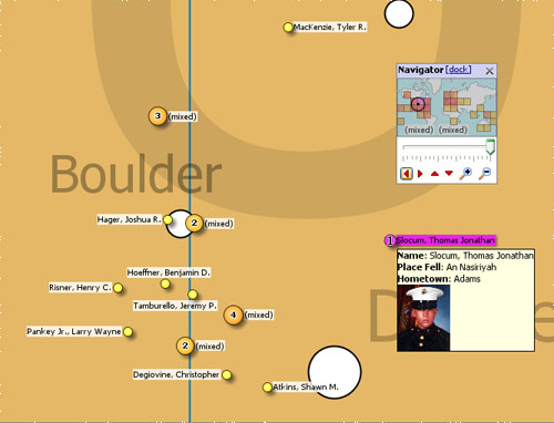
Labelling is displayed for all unaggregated records. Selecting a record can also trigger the display of Tooltips, which cam include associated images. Tooltips are configured for all views using Settings > Tooltips > Fields from the Main Toolbar.
Click the ‘Navigator’ button to show a small map navigation and view control window that can be placed anywhere on screen. Moving the zooming slider, or clicking the (+) Zoom in, or (-) Zoom out icons increases or decreases the magnification, which reduces or increases the coverage area shown in the thumbnail map framing window. Clicking the red vertical and horizontal arrows in the Navigator moves the small framing window around the thumbnail map. The thumbnail map in the Navigator shows a heat map of record density, and selected areas in blue. Click and drag the red thumbnail map framing window in to move around the main map.
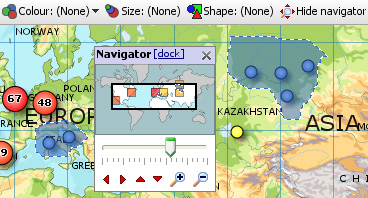
The Map View Tools drop-down menu provides options to define maps and control the display of markers.
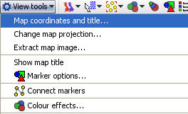
Map coordinates and title- displays the Configure Map dialog used to specify the title and coordinate fields (columns) to be used to place records on this particular map. With the correct map displayed in the view, select the fields to use as coordinates.
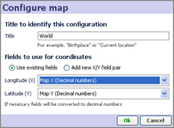 | Use existing fields- if your data sets already have columns of decimal coordinates, fully-populated or not. Most Visokio maps, including the default World map, support decimal numeric values available free from Google Earth. |
For more detail on map coordinate systems, and creating/transforming coordinate systems, see the Knowledge Base section on Maps & Coordinates. [53]
Change map projection- (not shown with Google Maps) used to create or refine coordinate systems for maps/backdrops that do not conform to the default Mercator projection decimal latitude and longitude system. This is most commonly the case with scanned images like floor plans, sports fields, some city and road maps, etc.
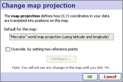 | Override, by setting two reference points- ticking this option launches the Change Map Projection wizard to define or refine the coordinate mapping. The wizard displays the map, with three advanced options to define or re-calibrate the mapping by 1) positioning corner reference points of known location, or 2) distributing the range across the entire map, or 3) using one-to-one mapping of pixels to coordinates (the default). |
For more detail on using these 3 options to determine the display of your data on a given map or image, see the Knowledge Base section on Changing Projections [54].
Extract map image- (not available with Google Maps) allows you to export a copy of the embedded vector map as an image file
Show map title- (not available with Google Maps) when ticked, displays the map title(s) in the upper left the map, in orange font as shown in the examples at the top of the page.
Marker options- clicking launches the Marker options dialog, very similar to that used in the Graph View [52]. This dialog enables you to configure how markers on displayed on the maps/scanned images you are using as backdrops for your data.
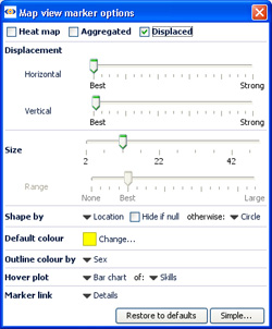 | Heat Map- (not available with Google Maps) shows density plot of records on a grid. Useful for plotting very large numbers of records that overlap a great deal. |
Displacement- (not available with Google Maps) changes the amount of displacement vertically and horizontally to improve access to data points for selection and linking.
Size slider- changes the absolute scale for marker sizing to increase or decrease all marker sizes
Range slider- (greyed-out unless the Size option is set to a field) changes the magnitude of relative sizing (see Size below)
Shape by: (not available with Google Maps) selects the field (column) whose values will determine the shapes plotted (same as Shape: toolbar pick list below) with additional options to specify the display of markers of records which are null (blank, not zero) in the selected Shape by field. In Simple mode, the Default shape to use when no Shape-by field has been chosen can be set.
Default shape/colour- selects the default colour of markers when no other colouring options are set.
Outline colour by: (not available with Google Maps) adds an outline of another colour, based on another field. For example, if 'Sex' is used, this command would put a blue outline on the dots representing Males and a pink outline on the dots representing Females- assuming that you have assigned the those colours to the values 'Male' and Female'.
Hover plot- (not available with Google Maps) sets a pop-up display of either a pie or a bar chart whenever the user hovers on a marker, aggregated or not. When set, you can select the field (column) to be charted using the pick list at right, which is otherwise greyed-out.
Marker link- (not available with Google Maps) selects a link to display when markers are clicked (one record only). Pick (None), Details, or one of the links already configured in the file using the Settings > Links wizard accessed from the Main Toolbar.
Connect markers- (not available with Google Maps) similar to the option available in the Graph View [52], opens and expandable sub-menu. Use of these options with the Map View is documented here. [55]
Colour Effects- (not available with Google Maps) launches an extensive menu of options to modify the display of the map/backdrop:
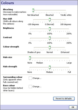 | Bleaching- reduces the intensity of the map image, making the markers more distinct.
|
{update to 2.5 on progress}
Omniscope allows you to use embedded vector maps that work offline, or online mapping services, such as Google Maps. Users can change from one zooming map background to the other within the Map View. Omniscope includes a wide selection of freely dowloadable vector maps (world, county or city level) which can be downloaded automatically and added into any file. Coordinate data in your data set is automatically plotted on maps or scanned images, such as floor plans. Markers can also be placed manually and Omniscope will automatically capture the coordinates to your data set. For more information on freely downloadable maps and how to use them, please visit our Maps Library [56].
Omniscope permits you to have multiple map views, using either vector maps (work offline) or Google Maps backdrops (work online only). The example below shows both vector and Google Maps being used to display the same coordinate data, visible in the Table View at the bottom (click image to see larger version in a separate window).
 [57]
[57]
Map Views allow easy zooming, selection and filtering of records (rows) based on location. You can use mouse mode controls and zoom options to manage the display, and then select groups of records on which to perform Move or Keep power queries.
To learn more about navigating, selecting and filtering, see the User Guide section Using the Map View [13], and the KnowledgeBase sections on Maps & Coordinates [58].
You can add embeddable vector maps to your local library and files from the File > Open map command, which is also accessible from the opening desktop Tasks menu. Downloading a map from our Maps Library [56] adds it to your local collection. If you use the map in a file shared with others, and they do not have the map, it will be automatically downloaded for use in the file. It is also possible to embed maps in files if necessary.
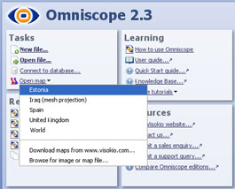 |  |
You can use any type of scanned image as map- floor plans, sports fields, logistics and supply chain charts, etc. To learn how to calibrate coordinates for display on scanned images rather than map projections, see Changing Projections [59] in the Knowledge Base.
Every map defined in Omniscope requires you to specify two columns to contain the Longitude (X) and Latitude (Y) coordinate values used to plot the records (rows) on the map. There are currently three ways to add geographic decimal coordinate (longitude and latitude) column values to your data for map displays;
1.) Locate your records in Omniscope using the free Visokio world, country and city vector maps- just select each record in the table view and place the markers manually to generate the coordinates in new fields (columns) automatically;
2.) Look up missing coordinates using online sources for finding coordinates such as Google Earth (and often Wikipedia). In Google Earth, look up the missing places, set a placemark, then read off the placemark coordinate values, then type or cut-and-paste the two Longitude and Latitude values into Omniscope columns;
3.) Merge the columns into your Omniscope data automatically using a merge file [60]. To merge in coordinate columns for capital cities or geographic centres of countries, we supply free 'By Countries' [60]merge file containing these columns. We also supply a free 'By Cities' [61]merge file containing coordinates for about 60,000 of the world's largest cities. Free merge files 'By post code' [62]are also available for the UK and the U.S., and a growing number of other countries as well. Other free and licensed reference merge files may be available from data vendors in future.
To learn more, see the User Guide section Using the Map View [13], and the Knowledge Base sections on Maps & Coordinates [58].
Map projections define how the (X,Y) coordinates in your data set are displayed over imported images/maps used in the Map View. Omniscope allows you to calibrate or define coordinate grids on any kind of map, photo or scanned image imported for use as a map. For example, you can use an online mapping service to zoom into a specific area, then take a screenshot and use that image as a map background in your Omniscope file.
The Omniscope Map View [63] Toolbar View Tools menu (or the Configure Map View wizard in DataPlayer View) includes the command Change map projection. If your X,Y coordinate columns in your data set is consistent with the default projection for Omniscope maps (Mercator projections using decimal latitude and longitude coordinates as used by free services such as Google Maps/Earth), you will not need to use this command. However, if you are using a scanned image as a background map, or maps that are not consistent with the Mercator standard projection, you may need to tick the Override, by setting two reference points option.
This dialog allows you to configure and refine how coordinates in the data file will be positioned on your map. There are 3 options:
Option 1. You know the coordinates of specific points on the image - If, for example, you have imported a screenshot image of New York's streets (from Google Maps or other online zooming map service) and you have coordinates in your data set in some form of grid reference (such as latitude and longitude, which on a small scale are linear), and you know the coordinates of reference points, (say, two street intersections) that are diagonally apart (looked up in Google Earth, for example), you would use Change Reference Point Coordinates 1 and 2 to ensure points in your data set will plot in the correct location. Drag the two reference points on your image to where each of your reference crossroads are located, then click the Change Reference Point buttons to enter the correct coordinate locations for each crossroad.
Option 2. You want the points distributed across the image- for example, you might have a data file of events during a game on a soccer pitch, and have imported a picture of the pitch to use as a map. You place corner events in two opposite corners of the pitch image. The coordinate system in your data file could be arbitrary, but assuming events happened across the entire pitch, you would click Distribute data points across map and the application would work out the transformation so as to "normalise" the points correctly.
Option 3. You want the data points to map to the pixels in the image (default). To revert to the default setting, where data coordinates correspond to pixel positions in the image, click 1:1 (pixel coordinates).
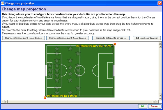
This section demonstrates how to use the Connect Markers option in the Map View to draw a path around the map. You can download this example file showing a holiday around the world here. [64] The various display commands on the expanded sub-menu are documented below.
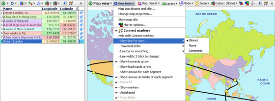
Start Omniscope and select File > Open map, then choose World. A new empty file will be created and opened, showing the Map View and the installed World Map, ready for adding markers.
From the Map View View Tools menu choose Connect Markers. Since you don't have any markers yet, you won't see any change.
From the Mode drop-down in the Map view, choose Place marker mode. The mouse pointer will change to a cross-hair when over the map. Move to the first location in the trip (for example, London in the UK), and click the left mouse button. The Add record dialog will appear. Type in a summary of this location, and press Enter or click OK. For example, 'Depart London, UK'. Move the mouse pointer to 'hover' over this marker. You'll see a Tooltip appear with the text you have entered.
Now click the Map View Navigator button to show the Map Navigator, and use the controls to zoom in and pan around until you can see the next location accurately. Click to add another marker, and enter the description. For example, zoom into Hong Kong and add a marker with the text 'A few days in Hong Kong'.
You'll see a black line joining the marker from the previous point. Carry on zooming into cities and adding markers and text until you've finished the path around the map. You can add more information by adding fields (columns) using Data > Manage Fields [35] to add fields (columns), and then entering data into your new fields from the Table View [65], which you can open using ![]() Add View.
Add View.
Click the Map View Mode drop-down again and change to Zoom mode to avoid accidentally placing markers. Open the Mode drop-down again and click Zoom to fit map. You'll see the entire trip with a black line joining the markers. Hover the mouse pointer over a marker and you'll see the text for that point. If you don't like the "line/curve smoothing", you can adjust or turn this off from within the View Tools menu.
Traversal Order (showing an omni-directional path) By unticking Time series (connect markers by X axis), you can choose to draw the lines in a different order than dictated by the X axis. If you are plotting data based on criteria other than time, configure the Traversal order field appropriately.
Show moving average: None; Simple & Exponential- If you have many data points in each time series, you may wish to try showing a moving average, by choosing Simple, Exponential or other data smoothing options on the sub-menu.
Line/curve smoothing- By default, lines are turned into curves while preserving data points. In other words, curves are drawn between the data points. Depending on your data, this may be inappropriate. You can disable this using the Line/curve smoothing sub-menu. Alternatively, a second form of curve smoothing is provided, which does not pass through the data points. Untick Curves pass through vertex points to use this option. Both forms of smoothing can be adjusted for amount of smoothing using the Smoothing amount option.
Line width-By default, lines are shown 2 pixels thick. Use the slider to change this any value between 1 and 25 pixels.
Arrows: Show forward arrow; backward arrow; arrows for each segment; middle of each segment-adds different kinds of directional arrow heads to the line segments displayed
Coloured- By default, if you have multiple lines displayed, these are coloured according to the values in the Category field. You can disable this and show only black lines by deselecting this option.
Show markers- Hides or reveals the markers within the plotted lines (to resize markers, see Marker Options on the View Tools menu
Anti-aliased- Smooths the way the line is displayed
Show labels- By default, text labels will be shown beside each line if you have multiple lines. By de-selecting Show labels, these will only be shown as you move the mouse pointer over a line.
The section on Time Series [37] also covers advanced options for the Time Series > Connect Markers functions, most of which are the same in the Map View.
All Visokio applications come with embedded world maps (Mercator projection) and will plot records (rows) according to decimal latitude and longitude coordinates contained in two selected fields (columns) of your data sets. If your data does not yet contain map coordinates, you may be able to add them automatically using a Merge File, or you can populate the fields manually using Visokio maps and the Place Marker process [49].
This brief tutorial explains how to:
|
|
Opening MapsChoose File > Open map and choose any map from the list to create a new, empty .IOK file showing only the chosen map. You can add maps to your list from the Maps Library [48]. |
Zooming inInitially, the Map View opens in Zoom Mode,indicated by the magnifying glass mouse cursor. In Zoom Mode, you can click and drag the mouse to zoom in and out on selected areas of the map. To zoom in, click on a central point of interest, or click and drag (press and hold a mouse button while moving the mouse) to draw a rectangular 'zoom' box over an area. To zoom out, right-click anywhere on the map and use the slider or the (-) Zoom out |
| Viewing layersOmniscope maps have many layers that can be either hidden or shown. Layers contain feature-specific detail available on the maps, such as 'Capitals' or 'waterways'. Note: some of the details in some layers are only visible |
 | Managing layers Tick or untick the boxes next to any layers you wish to display or hide. For example, at left we've removed the physical layer (which includes relief shading). The result is to display the map coloured by political boundaries rather than topology. |
| Using the Map NavigatorClicking on the Map Navigator icon launches a floating tool that speeds focusing on specific areas of the map. The slider and magnifying glass tools manage zooming in and out. You can grab the sides of the mini-frame to move it and change the scope of the display. The four red arrows below move the focus frame in the direction they point. |
| Placing MarkersMissing map coordinates associated with a given record (row) can be added/changed manually. On the View Toolbar, click on the
|
Use | |
| Selecting RecordsClick on the |
| Viewing DetailsSelect an area on the map containing one or more data points. The area will be framed in blue. Click on Clicking on a single marker will display details for just that record |
The Venn View is based on the familiar Venn diagram. This view enables visualisation and filtering on overlaps between up to 5 different named query data sets or subsets, which must first be pre-defined as Named Queries [22]. Notice that the number of records (or other measure specified in Value/Function) not included in any selected set/subset is displayed upper left after the heading 'Outside'. In the HR example below right, the median age of all the staff not included in one of the selected subsets is 42.
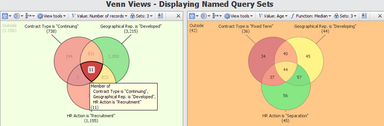
![]()
Venn View Toolbar View picker, Data Subset selector, Aggregate options drop-down and the show Details all function the same as they do in all the views. View Toolbar options unique to the Venn View include the upper-pane View tools options, the Value: menu to specify the values to be used, and the Sets: menu to specify the existing Named Query data subsets (maximum 5) for which Venn shapes will be displayed.
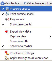 | Venn View > View tools Preserve aspect - (default) locks the shape of each circle to remain a circle. Unticking this option allows the Venn shapes to distort to reflect the intersections. Paint outside space - colours the background outside the Venn shapes, which can improve visual impact especially if there are unselected records being displayed upper left under the heading 'Outside' Play sounds - try it, you might like it Show zero counts - displays set names and intersection counts even if zero.
The rest of the options in the lower panes are common to the View tools menus for all views and are documented here [2]. |
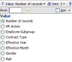 | Venn View > Value: {Function} Use this menu to select the values for which the counts are displayed inside the Venn shape representing each data set/subset. Notice that text columns are not shown. Counts only are available for category values. If you select numeric value, an additional Function menu appears allowing you to specify the calculation applied. (see example of average age above right)
Find: shows subsets of field (column) names to shorten the list Sort: orders the field (column) names to speed selection |
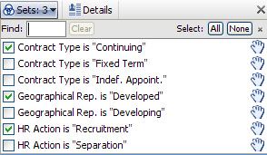 | Venn View > Sets: (number of sets selected) All of the Named Queries which define subsets are available here for selection and display as Venn shapes, up to a limit of 5. Drag the hands at right upwards or downwards to re-order the list. |
The Details View can display all of the information about a record in Omniscope, with very flexible branding, text formatting and image display options. Can also be used as an editing form, allowing data entry and corrections by anyone with basic keyboard skills. Whenever a Details View is open, the Details display for individual records will show in the open view, rather than the pop-up or Side Bar panel details displays.
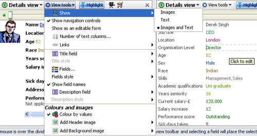
The Details View toolbar contains a View Tools drop-down, a Highlight button (used to turn record highlighting in other views off and on) and the Slideshow, Add to Basket and [X] Close view commands common to other views. For more detail on highlighting and configuring slide shows, see Viewing Details and Highlighting [66].
Warning: If you have global record cycling enabled, and you turn off the Highlighting option, the record cycling will stop. To re-start record cycling, hover your mouse on the barometer to expose the global automatic record cycling menu, and click on the green forward arrow to re-start.
The View Tools drop-down menu contains many flexible options for configuring the Details View display:
Show - defines what to display; images only, text only or both. When there is more than one image set configured, you can select which images to show (they appear horizontally).
Show navigation controls - when ticked, displays a manual record-cycling slider only for the Details View. This is different from the automatic record cycling which affects all views. Drag the slider forwards and back, enter a record number or use the green forward/back arrows. When ticked, the Sync(hronisation) option keeps the record cycling in the that Details View on the same record as the global record-cycling.
Show as an editable form - when ticked, for each record, all fields are displayed in a single column with the values in individual text editing boxes, as shown in the example above right. This mode is used to facilitate data entry and correction using a single, easy-to-understand interface that anyone can use.
Number of text columns - drag the slider to the number of columns you want to use to display the text/field values you wish to show. The default is two columns with coloured values following field names as shown in the example below:
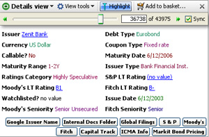
Links - similar to the command used in other views, this displays a pick list is used to assign which values will be underlined and launch associated links from the Details View. In the example directly above, the 'Issuer', 'S&P', 'Moody's' and 'Fitch' field values have been assigned links, and therefore show underlined. In the Details View, at the top the top of the links menu is a Configure links buttons option:
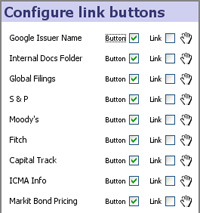 | As shown in the example above, for each link where the 'Button' option is ticked, and action button is displayed in the Details View. Ticking on the 'Link' option adds an underlined link bearing the link name to the bottom of the display, as an alternative to the button. Use the 'hand' drag handles to move Buttons/Links up or down, re-ordering them in the display from left to right as shown above. |
Title Field - selects a field (column) value to display in the upper left-hand corner of the view window. If you display a field as a Title, remember to untick the Title field in the fields pick list (see below) to avoid displaying the values twice.
Title Style - enables you to apply text styling (fonts, font face, colour and alignment) to the Title field display.
Fields - a pick list appears allowing you to tick/untick fields you wish to show/hide; drag the hands up or down to change the order (Note: you will only see these when ‘Text’ or ‘Images and text’ is chosen in the ‘Show’ menu).
Show field names - when ticked (default) displays the field (column) names prior to the values. Untick to suppress the filed names.
Description field - selects a field (column) value to display at the bottom of all other fields. Used to display longer text entries that do not wrap well if displayed in the columns with other, shorter field values. If you display a field as a Description, remember to un-tick the Description field in the fields pick list (see above) to avoid displaying the values twice.
Description style - enables you to apply text styling (fonts, font face, colour and alignment) to the Description field
Colour by values - when ticked, colours category values according to the colours assigned to each value, and numbers/dates by the scale reflecting the range of values (default : low=red to high = green). Text fields are always displayed in black.
Add Header/Background Image - used to include logos and other faded backgrounds in the display.
The other commands on the Details View Tools menu are common to all views and documented under View Tools. [2]
The layout and sizing of the image and text spaces in the Details View is controlled using a divider line which you can find by hovering the mouse over the divider between image and text. When you do this, the frame divider will appear. Click and drag the divider to get the proportion of image to text area you want. Click the frame divider switch button on the right when the divider appears and the orientation will switch between horizontal and vertical.
Suggestion: Omniscope has powerful image re-sizing and management features. Be sure to experiment with allocating more space to the images to optimise the display in the Details View
The Web View is one of the 12 standard views available in Omniscope. It differs for the other views in that it is not intended to depict all of the data in the data set. Instead, it is intended to broaden the reach of the Omniscope file to other related content and services available on the web.
As with other views, you can add a Web View to the display by switching one or more existing views to be Web Views (by clicking the view name and choosing Web View in the View Chooser) or by adding a new Web View to the display using ![]() Add view on the Main Toolbar
Add view on the Main Toolbar
You can have any number of Web Views open, with each pointing to a different address (URL) on the web:
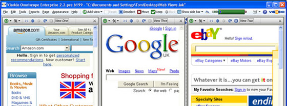
The first time you open the Web View, it will show the Omniscope default static page (the Google homepage). "Static" means this view won't update when you filter or navigate in Omniscope. Omniscope Web Views work just like web browsers. You can enter a different address in the address bar, or follow the links on the page displayed to change the current page. You can resize the windows to be quite small. Omniscope can switch the screen display of the web page to a style intended for small screen devices.
If you save the .IOK file and later re-open it, any static Web Views will re-open showing the same page that was showing when you saved the file. There is no such thing as a "home page" with the Omniscope Web View. Instead, Google is the default page if you've never opened a Web View before, and each Web View will re-open as it was saved.
A dynamic Web View is one that is automatically synchronised with the rest of Omniscope. When you select specific data in another Omniscope view, the Web View will reload to show a relevant page as defined by the selected link. You can't enter a different web address into a dynamic Web View. To change a dynamic Web View back to a static one, change Link or Web service to "(none)" in the View Toolbar.
There are two types of dynamic web view: link-based and web service-based. Both are used for showing web pages containing information about a single record (link-based) or groups of records (web-service based). When you highlight a record in Omniscope, an open link-based Web View will update to show the linked page for the highlighted record. If there is no record selected/highlighted in any Omniscope view, link-based dynamic Web Views will remain blank.
In Omniscope, a highlight is set whenever you select a single record, such as a single row in the Table View. In the example below, selecting the record of a specific casualty in Iraq displays a personal memorial page for that soldier in the link-based Web View:
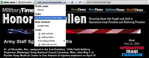
To create a link like this in an Omniscope file, choose Web View> View Toolbar > Link > (Tools)/Add web link. This allows you to define the link and associate that link with that Web View. You can administer all the links in your file from the top-level Settings > Links [67] menu.
It is possible to define much more complex data-driven links. For example, you can use two or more field values as parameters in a link like this one:
http://myIntranetServer/addressBook?firstName=[First Name]&lastName=[Last Name]
where 'First Name, and 'Last Name' are fields in the data set.
Omniscope has a number of preconfigured links built in, which saves you having to figure out the link syntax for common websites offering free web services. See Using Web Services in the Web View [68]
Web views are also used to display the results of dynamic requests for web services. Some free web services, such as YouTube and Google Maps, are already configured. If your file includes a collection of video clip identifiers recognised by YouTube, selecting a clip from your Omniscope 'video jukebox' will play the corresponding clip in a Web View as streamed from YouTube:
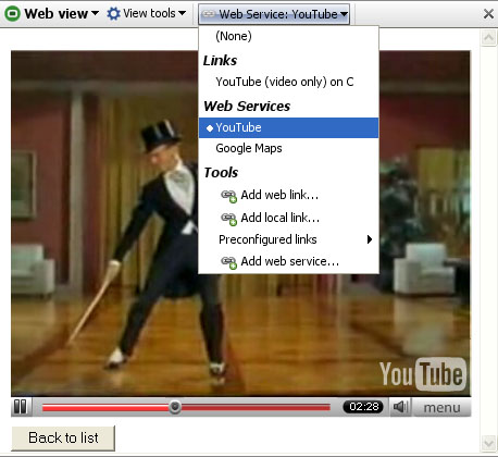
You can also add any custom Web Service to your file. As with Links, you must pre-define custom Web Services configurations using the Main Toolbar Settings > Web Services menu, then use the Web View selector drop down to the right of the View Tools drop-down to link that Web View with the selected web service.
Connections to web services that accept a series of inputs (or a table), rather than a single value/text string, are less easy to implement, since they require a specific web server page implementation. Examples of multi-record Web Services already defined in Omniscope include popular mapping services, such as Google Maps.
Multi-record web services links to Omniscope work by submitting an HTTP POST to the web service page containing a series of record IDs. This is equivalent to submitting a form listing all the record IDs. This functionality allows you to program server pages that accept a list of record IDs in an HTTP POST request and provides any further information associated with those records in HTML, in the HTTP response. You can also configure the maximum number of records in a web service post (the default is 100). This allows you to restrict access to the server page to only moderate requests, especially useful if allowing users to retrieve 50,000 price graphs at a time might be undesirable. At present, you can only configure a single-parameter web service post. If you envision a solution that requires a tabular, multi-field post, please contact us.
We provide a simple example 'echo' page which can be used to test your configuration and to understand the results. This is the default page when adding a Web Service. To see the test echo service, go to Settings > Web Services > Add web service and click OK without making any changes to the defaults.
After adding a web service, depending on how it was configured, you may need to select it in the Web View using the Link > Web Service selector to the right of the View Tools drop-down.
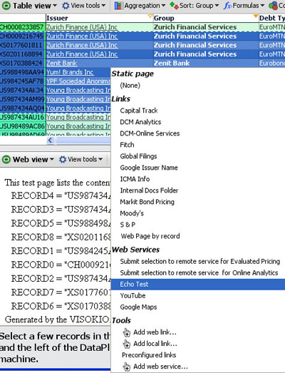
Web Views pointing at Web Services rather than links will show all records currently included by your filters. If you then make a data selection in another view (such as the Pie View), the Web View will show only the selected records. When you clear your selection, the Web View will return to showing all the records included by your filters.
To use the Echo test, first filter down to, or select, no more than 100 records using Side Bar filters and/or using Select, Move & Keep power query sequences in other views. Once the selected number of records falls below the threshold, Omniscope creates a form submission with form keys "RECORD0", "RECORD1", "RECORD2" (etc.) and posts the form values to the configured server for the selected Web Service. You will normally see the results of the POST returned in the Web View.
The Web View, like other views, is configurable using Report Pages. You can, for example, create a Report Page with 3 Web Views, and another Report Page with just a Table View and one Web View, then switch between the two. Omniscope supports opening any number of views and managing the positioning of these views through flipping individual panes using the 'flip' icon command on the view divider.
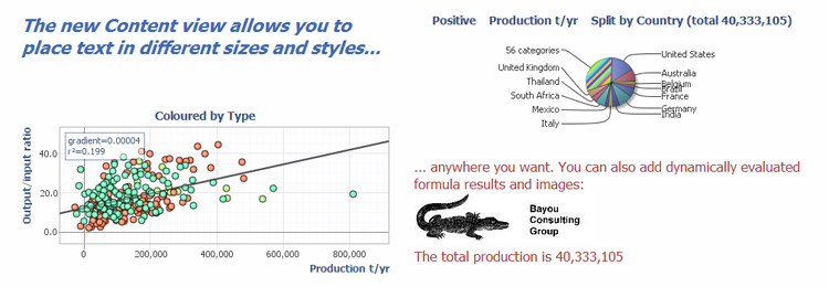
Like other View Toolbars, the left-most part of the Content View Toolbar contains the View and Data Subset selectors, and the Aggregate options drop-down. The View Tools drop-down begins with commands unique to this view, followed by commands common to all views.
![]()
To the right of the View Tools menu are the Format and Edit options drop-downs specific to the Contetn View. Use of these is discussed in the sections below.
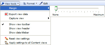
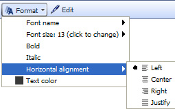
| Insert - Click to enter Edit mode, which reveals the Insert drop-down containing options to insert a wide variety of content inside the view display using the wizards to assist you Commit - Once you have completed inserting content, click to make your changes persistent in the file. You can still change the formatting of the content you have inserted. Cancel - Reverts the content to the last committed state.
|
Edit Annotation [69]
Web and File Link [70]
Formula [71]
Aggregate [72]
Subset: Filtered data [73]Aggregate [72]
Subset: Filtered data [73]
Content is available from Add view on the toolbar menu.
To see how to edit /change the font/ insert image .... to the Edit box please click on this link: Text Editor [74].
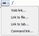 | The user can link any web page or file into the Content window. |
Here is an example of how a user can create a link :
| Select a link (Link to tab for example) a pop up with all tab’s name will appear on the screen:
The user can select any tab wanted ( DataManager), then press OK to validate. A new pop up will appear asking to enter the text that you want to display. Omniscope keep the name set by default. The user can at any time click on it, and change the name of the link. After pressing OK, the link will appears in the content window, you will have to click on the link to be redirected to the Tab. Same Principal if you want to create a link for: Web page, files, or create a command list.
Back to the Top [75]
|
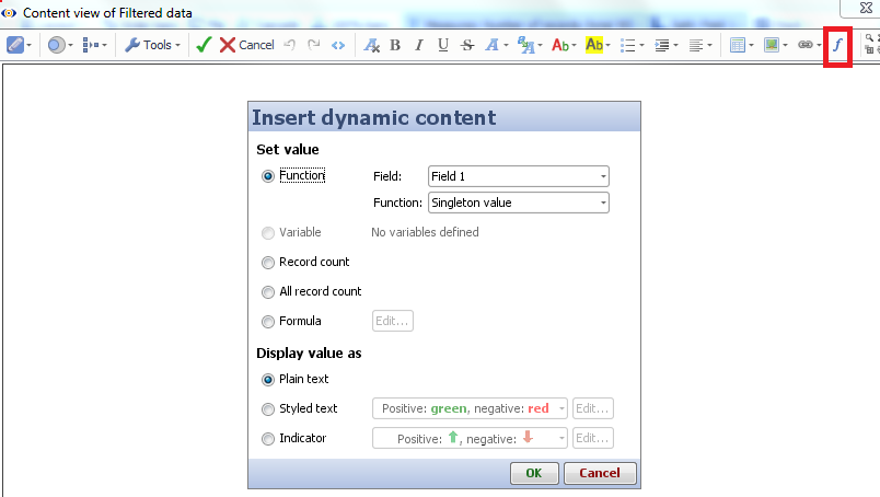 | The user is able to insert a formula in the content view by clicking The user can set value by selecting: Function /Variable /Record Count /All Record Count / Formula The user can also display the value as Plain text / Styled text or with Indicator
Back to the Top [75] |
Tools gives also the possibility to the user to Create:
-Header/ Footer …
-Modify the edge
-To export the data-Save a copy into the clipboard
The user can reset all modification at any time by selecting: Reset view setting’s option.
The user can apply the setting created to all Content views created in any tab by
selecting: Apply to all Content view’s option.
Back to the Top [75]
(Tools menu's option) | 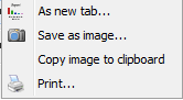
(capture view's option) | 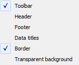 (Toolbars and style's Option) |
The user can aggregate any data when selecting the option Aggregate.
Back to the Top [75]
The user can aggregate any data when selecting the option Filtered Data.
Back to the Top [75]
Dial View allows you to create three different kinds of interactive dashboards. Provides familiar representation of relative magnitude of values drived from specific columns in the data set. This makes it easier for end users to view the results at a glance. Dial view itself is highly customisable. For example, you can specify the maximum/minimum range, create coloured zones etc.
Please note that dial alerts, range and zones settings are set for each individual value field. For example, if you set your dial alerts, ranges and zones and then switch your value field to something different than your settings will disappear. However, when you change your value field back to a field that previously had alerts, range or zones set, then the Dial view will restore them.
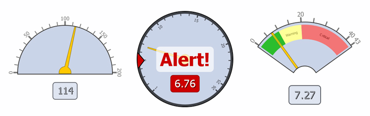
Dial View toolbar has generic options just like other views such as View changer, Subset, Aggregate and the View tools.
![]()
Dial View toolbar also contains options and settings which are specific to the view itself. These are described below.
The view tools is available in all other views and contains general options which are available in other views, but also options specific to Dial View.
|
| Margin: The slider allows you to adjust the space between the a particular dial and the view edges. This can allow you to make the dial smaller without having to adjust the dividers between the view. Show label: Ticking this option shows the quantity value based on the Value field. Show percentages: Ticking this option allows you to show the dial range in terms of percentages. Animated alert: This option only takes effect, if alert has been set, and the alert the condition has been met. When this option is ticked the alert text on the dial will flash. Dial background: Allows you to specify the background colour of the dial. Please note that this option doesn't change the view background, but only of the dial itself. Paint dial background gradient: If this option is ticked, then the dial background is painted with a gradient. Gradient is painted using the dial background colour. Needle colour: Allows you to specify the colour of the needle. The rest of the options are standard throughout the views, click here [2] for further details.
|
Style option allows you to choose between three different type of dial styles. This list may increase in the future versions.
|
|
|
The range settings allows you to specify the minimum and maximum values for the dial. Once you have specified the range values the dial view will use that that to show represent the values. If the value falls outside the range of the dial, then warning text is shown.
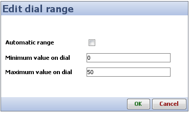 | Automatic range: When this option is ticked, the values for the minimum and maximum are automatically calculated by the view. These values will be determined by the underlying data being displayed.
Minimum value on dial and Maximum value on dial: These two options only become enabled when Automatic range is unticked. These allow you to specify your own minimum and maximum value settings. This can be helpful when you want to limit the values of the dial to a certain range. |
Dial view allows you to set your own alerts when certain conditions are met. For example, if you are monitoring sales target, you could have an alert that tells you once 50% of the the items are sold provide some kind of visual notification. You can also use the multiple alerts functionality of the dial view to add further alerts. However, dial view will only show the text of the first alert that has been met. For example, continuing from the previous example, if you have an alert set at 50% and another at 70%, but if the sales have gone beyond 70%, then the dial view show the alert for 50% and not for 70%. Having said that you can from the alerts dialog change this precedence. When no alert condition have been met, but there are alerts set then dial view shows a white triangle on the edge of the dial to indicate where these alerts have been set. Below is a description of how you can add alerts to your Dial View.
When you click on the Alerts button you are presented with the following dialog. The edit alerts dialog allows you to add new alerts, edit existing alerts, remove alerts or change the precedence of the alerts.
| Add...: Allows you to add more alerts. Edit selected...: Allows you to edit a selected alert. Remove selected: Allows you to remove the selected alert. Up and Down: Allows you to change the precedence of the alerts. |
When you click on either Add or Edit buttons in the Edit alerts dialog you are presented with the Add/Edit Alerts dialog an example of which is shown and described below.
| Alert text: The text to display when the alert condition has been met. Alert position: The position of the alert (i.e. the position of the alert in terms of the range). Alert condition: The actual condition which is used whether a certain value is greater than, less than, equal to etc to the alert position. |
The zones settings allow you to set zones to sub-divide the values into different sections. Each of the sub-sections can be assigned a coloured zone and a label. This can be very useful when you have lots of values, and the values can be seperated into groups i.e Low, Medium and High. Below is a description of how you can add zones to your Dial View.
When you click on the Zones button in the View toolbar you are presented with the following dialog. From this dialog you can add, edit, remove and change precendence of the zones. This is useful when you have two or more zones are overlapping each other, as just like with alerts the earlier zones take precedence.
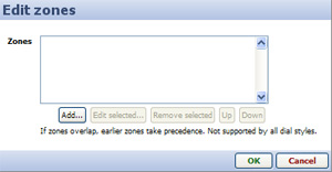 | Add...: Allows you to add a new zone to your dial. Edit selected...: Allows you to edit a selected zone. Remove selected: Allows you to remove a selected zone. Up and Down: Allow you to change the precedence of the zones. |
When you click Add... or Edit selected... buttons in the Edit zones dialog you are shown the following dialog which allows you to configure the zones.
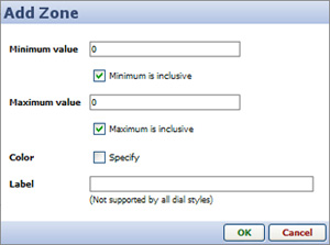 | Minimum value: Represents the minimum value of the zone. Minimum is inclusive: If ticked, means the minimum value is included in the zone. Maximum value: Represents the maximum value of the zone. Maximum is inclusive: If ticked, means that that maximum value is included in the zone. Color: Allows you to specify a colour for the zone. In order to specify the colour you first need to tick the Specify text box. Once you tick the box a colour button will appear next to it from which you can choose the colour. Label: Allows you to specify text to label the zone. This text is shown within the zone in the dial. Please note that this is not supported by all dial styles. |
The value field drop down which is also present in some other views allows you to specify what values to show within the view. By default this is set to Number of records. However, you can easily change this to a particular field. Depending on the type of field you select, a Function: menu will appear, allowing you to chose whether to display the sum, the mean, or some other transformation of the data. If you choose a function such as mean, a Weight: menu will allowing you to specify another field to calculate weighted averages of the values. Below is an example of the Value field menu.
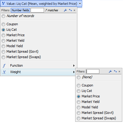
This view is no longer being developed. To use this view, you must enable Settings > Advanced > Show legacy features.
DataPlayers are standard .SWF Flash files which contain the data, multiple visualisations and intuitive query devices used to filter the interactive display(s).
DataPlayers can be created in any size, using either tabbed or simultaneous 'dashboard' layouts and any of many different view types. Interactive DataPlayers are exportable, universally-accessible Flash .SWF files for documents (PowerPoint, Excel and Adobe .PDF) and/or web pages. DataPlayers can be exported from Omniscope files using Professional or Enterprise Editions either directly into documents (with full interactivity), or as an HTML scripted target page, plus related Javascript, images and .SWF files within a single, uploadable folder, or or as standalone .SWF files for refreshing exported DataPlayer data sets by overwriting already posted .SWFs.
The Omniscope DataPlayer View enables DataPlayers to be created and displayed on tabs within Omniscope files. Omniscope .IOK files should be configured with dedicated tabs for one or more exportable DataPlayers. Whenever the data in the .IOK file is refreshed from its linked source or edited from any tab, the DataPlayer(s) will be updated within their Omniscope tab(s) using the newly-refreshed data and the persistent settings in the Views sub-menus.
The example below shows a tabbed configuration using each of the current views, one per tab. The Human Resources data set in the example below is the same as that included in the embedded 'How to use Omniscope.iok' tutorial file's DataPlayer tab. The data describes 111 employees of a fictional company with more than 4 years seniority.
Principal elements of all DataPlayers include:
View chooser buttons (tabbed display only) - each DataPlayer can contain multiple view types. Clicking on these tabs changes the view type displayed, the order of which you can determine by changing the order of the view types in the Views drop-down menu. Simultaneous 'dashboard' display is another Appearance option.
Query devices - the Omniscope Side Bar filter devices and value colouring/ordering settings displayed when the DataPlayer View is opened are replicated in the DataPlayer side filter panel. Like in Omniscope, clicking or sliding the filters in the side panel reduces the displayed record count, as displayed in the barometer at the bottom.
Slider - often, there are more query devices on the side filter panel than can be displayed vertically. DataPlayers where this occurs display a vertical slider to allow the user to access the query devices below the opening set.
Barometer - like Omniscope files, each DataPlayer displays a 'barometer' that indicates the number of records inside the DataPlayer, and the subset of those which are displaying given the current filter settings
Details button - this button can be used at any time to display record (row) level values according to the settings for single and multiple Details display.
Refresh button - like Omniscope files, clicking Refresh returns any filtered records to the visible data set, as confirmed by the barometer.
Within each view, drop-down menus can be configured to give users choices of fields (columns) to display, or no options at all.
Using the menu items available on the DataPlayer View Toolbar (see below), you can extend and refine the opening DataPlayer by adding other DataPlayer view types, and changing the Omniscope Side Bar filter settings to change the query devices available the filter panel generated in the DataPlayer(s) you are creating.
Warning: If you have more than 10-15,000 records in the 'Filtered data (IN)' data set when you first open a DataPlayer View, current limitations in Flash may interfere with full rendering of the initial DataPlayer. It is best to first define either an Aggregation or a Named Query (or both) such that the number of records to be encapsulated in the initial default DataPlayer is reduced to under about 10,000 (depending on row count and data complexity).
Caution: The DataPlayers displayed in the DataPlayer View are fully interactive, and thus it is possible to set filters, change selection drop-downs etc. just as end-users of the DataPlayer will. However, these changes are not persistent. The next time the DataPlayer View is opened and the DataPlayer re-generated, all settings will revert to the settings established in the View Toolbar Views settings menus, as described below.
The DataPlayer View Toolbar includes options to create exportable DataPlayers like the example above, using defined subsets, or even all of your data [76].
![]()
The DataPlayer View Toolbar View chooser, Data Subset selector and Aggregation drop-down menus work as they do in all Views. The functions of the other View Toolbar drop-down menus are documented below.
The bottom five commands on the View Tools drop-down are common to all Views and are documented here. Unlike most other views, View Tools > Capture View offers only the option of saving the DataPlayer on a new tab. Options to export DataPlayers to documents and web pages (with full interactivity) are located on the Save/export sub-menu.
| 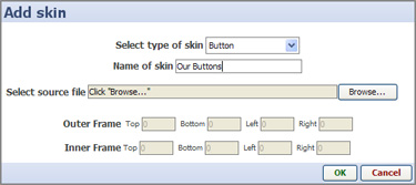 |
Create skin element > Add skin - DataPlayers are highly customisable. All of the principal elements of DataPlayers use skin elements that can be replaced with skin elements of your own creation. If you wish to add skin elements of your own to a file, select the type of skin element that you have created, give it the name you want to appear in the menus, select the source file containing your version, and set the Inner and Outer Frame limits. For more information on creating and using your own skin elements, see the KnowledgeBase article on modifying and creating skins [77].
All of the settings governing adding additional view types and the view-specific configurations of DataPlayers are on the Views drop-down menu.
Opening View:
| One of each View Type added with names:
|
Add, change, re-order (drag the 'hands' up or down) or remove DataPlayer view types from your DataPlayer using the commands on the Views drop-down menu.
Caution: It is good time-saving practise to re-order the DataPlayer view you are working on from last to first in the list. This is because each time you click 'Apply' or 'OK', the DataPlayer will be updated/re-generated with new settings, and the result will open to the first view/tab. Once all the views have been fully configured, you can re-order the views to suit your readers.
The Edit sub-menu commands (including re-naming each view) specific to each view type are documented on pages accessed from the links below (or from the User Guide DataPlayer View sub-menu links at the upper left of this page).
|
|
|
More view types are in development and will be added to future versions of Omniscope. Over time, the view types available in exportable Flash DataPlayer format will approach those available in the Omniscope project files. If you have urgent particular needs for evolution or addition of view types, please contact us [86].
Regardless of the number of view types in a DataPlayer (either in tabbed or simultaneous layout), options to display user-selected subsets of the records, either singly or in groups, for all of the views in a given DataPlayer are set using the Details drop-down menu.
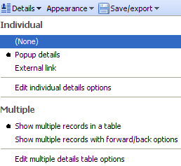 | Individual record (row) display options: (None) - no details display for individual records Edit individual details options - if 'Pop-up details' has been chosen, a three-tabbed options dialog will appear, documented here [87]. Multiple record (row) display options: Show multiple with forward/back - show 'card-deck' style secondary display enabling users to page through the pop-up details display for all the records selected. Edit multiple details options - depending on which option for multiple record display is chosen, a tabbed options dialog will appear, documented here. [87] |
The options governing the overall look and feel of the DataPlayer outside the individual view types are accessed from the Appearance drop-down menu.
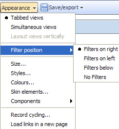 | Tabbed Views - display all one view at a time with buttons to switch views. Size - use sliders to set the width, height and filter panel width in pixels. |
Configuration sub-menus for Size, Styles, Colours, Skin elements and Components options are further documented here [88].
Record cycling - DataPlayers can be animated to 'step through' the highlighting of individual records, displaying Tooltips in some views
Load links in new page - if you have selected Individual details display option External link, tick this option to display the results of the link in a new tab of your readers' default external browser.
DataPlayers are separate Flash .SWF files which can be exported from Omniscope and inserted in documents and web pages with full interactivity. To use the document export options, your machine must have the relevant document-creation applications installed; MS PowerPoint and Excel, and either Adobe Acrobat Reader (free) or a .PDF Publisher.
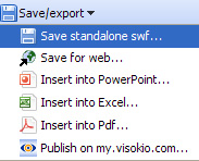 | Save standalone .SWF - exports just the main .SWF file, which can be uploaded with the same name to replace an older online version with a new version containing new data or modified configuration. Save for web - exports an model .HTML file containing <script> tags referencing a collection of files, image folders and scripts and the related, uploadable folder. All you need to do is paste in the <script> text and insert the <object> tags positioning the main .SWF file in the folder on the display page. Insert into PowerPoint - inserts the DataPlayer into a new or existing PowerPoint slide (only displays when presentation is opened in Slide Show mode). Insert into Excel - inserts the DataPlayer into a new or existing Excel workbook tab. Insert into .PDF - inserts the interactive DataPlayer into an Adobe .PDF document. |
Publish on my.visokio.com - you can post a DataPlayer on a blank page hosted by Visokio, then reference this page from your blog or send a link tot he page to your readers by e-mail.
More information on posting DataPlayers online [89]
More information on inserting DataPlayers in common documents [90]
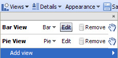
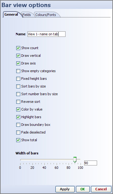
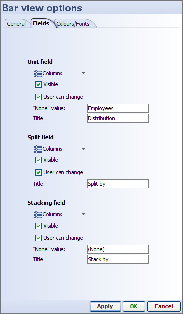
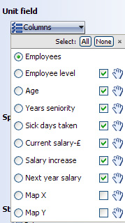
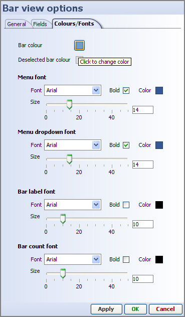
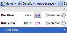
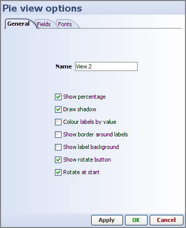
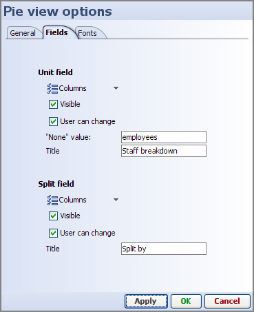
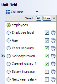
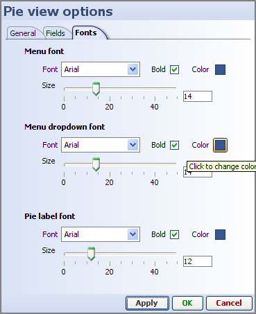
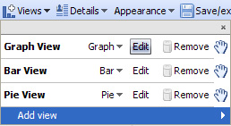
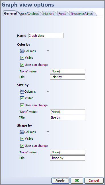
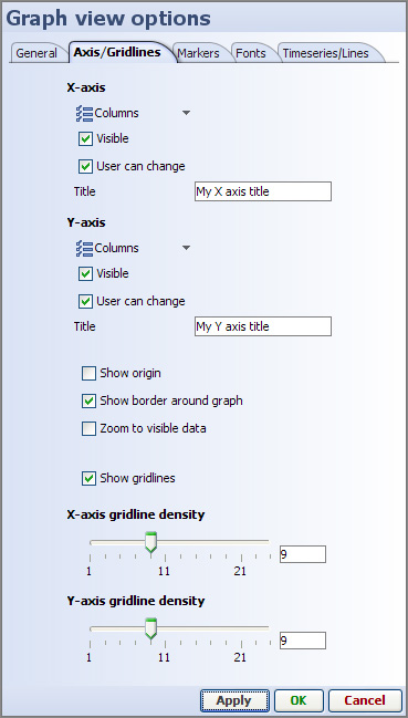
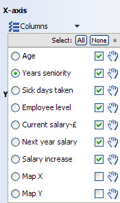
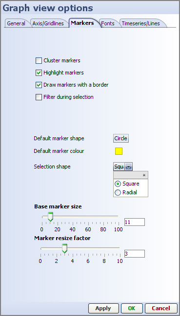
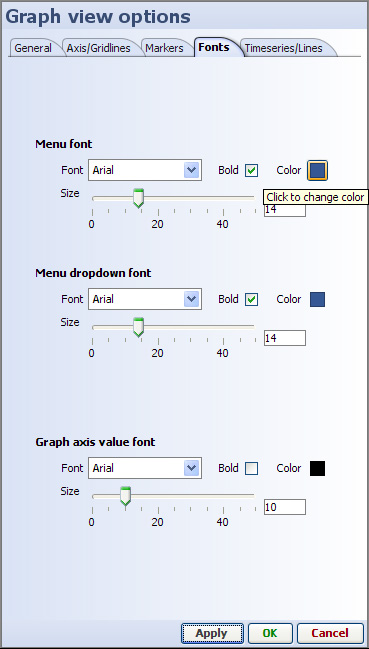
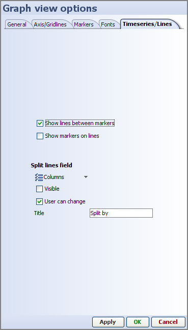
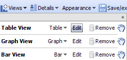
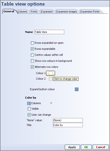
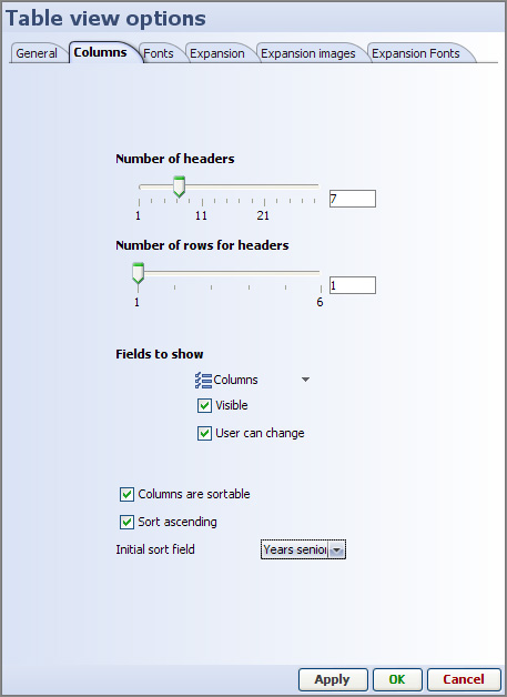
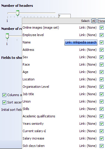
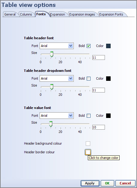
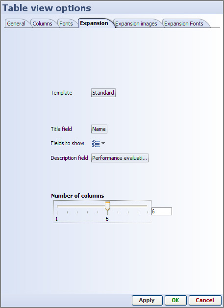
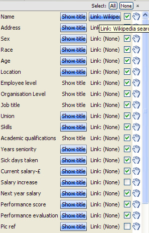
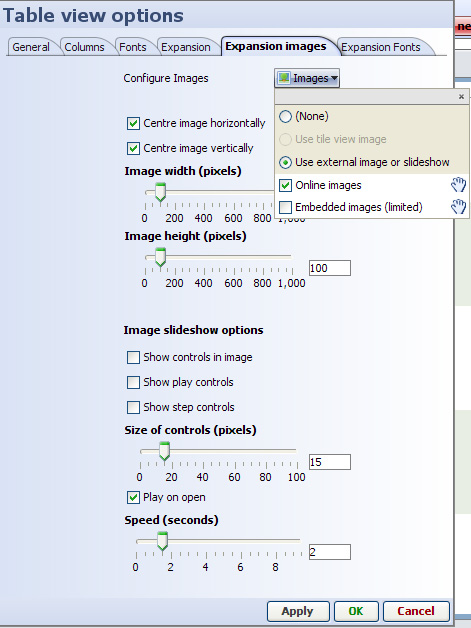
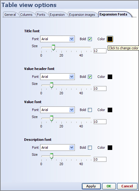
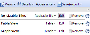
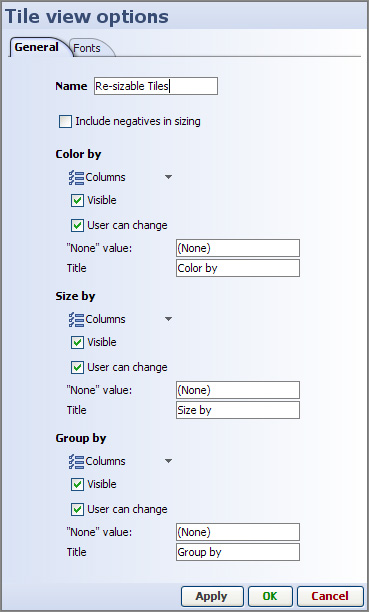
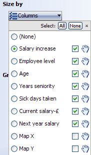
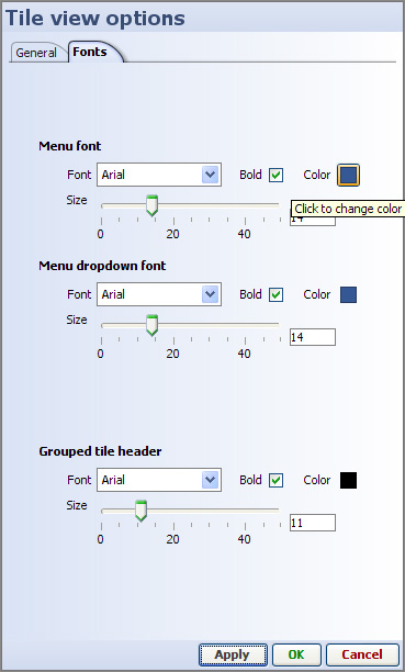
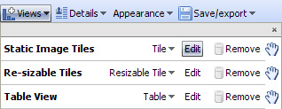
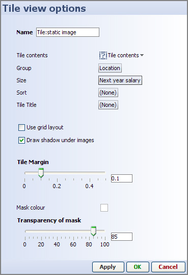 |
Name - the name you give will appear on the tab of the DataPlayer corresponding to this view. Tile Contents - specify either images from defined image sets or values from the data set to appear inside the tiles. |
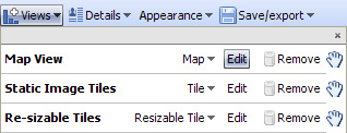

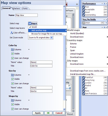
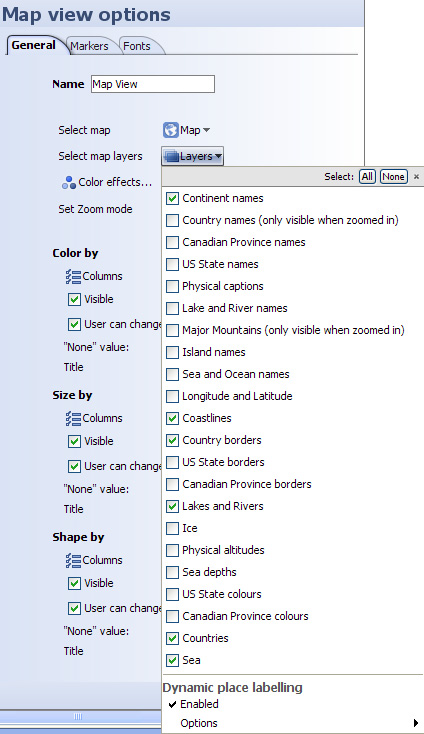
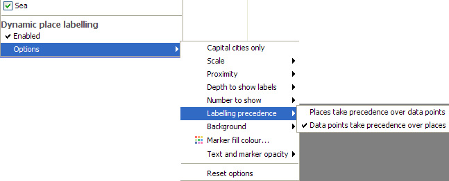
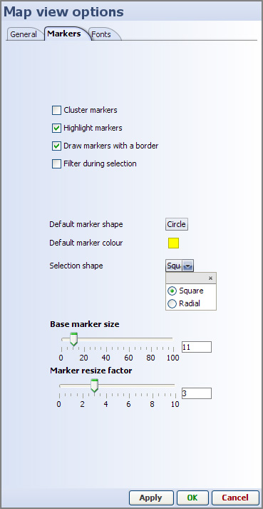
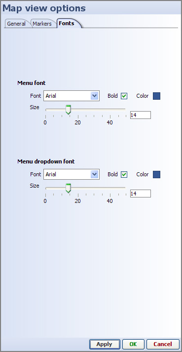
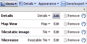
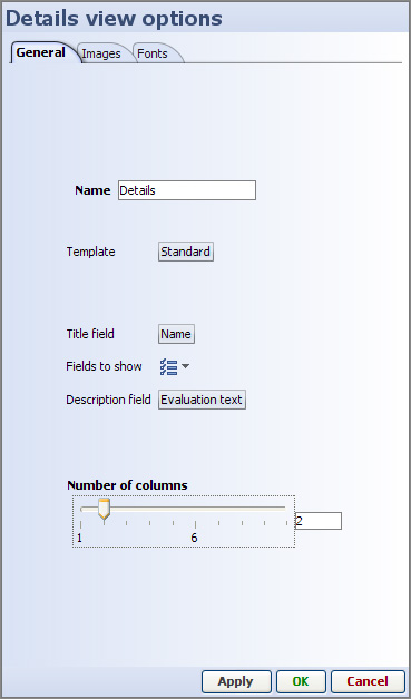
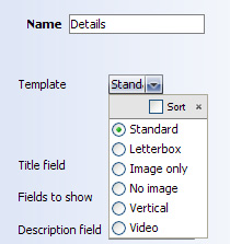
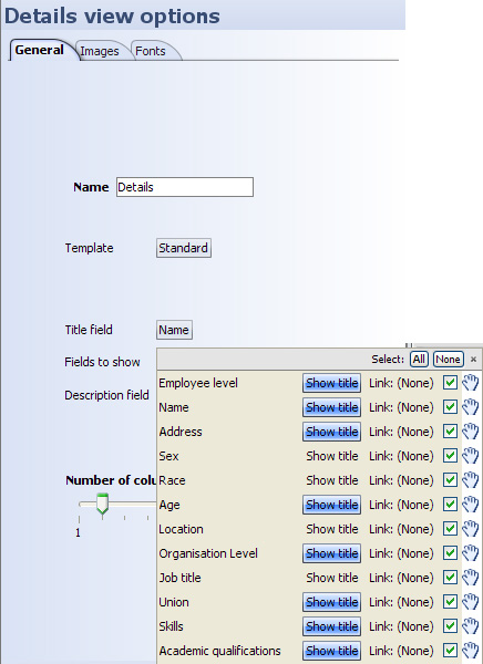
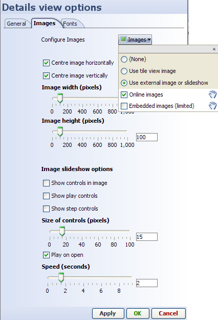
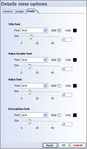
There are several options for configuring the display of the Details display windows that underlie each DataPlayer. Details display windows are not the same as Details View DataPlayers. Every DataPlayer view type includes a subsidiary Details window that responds to user clicks on the Details button.
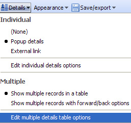 | Individual - refers to details for one record (row) only None - no details display window for individual records Popup details - details window will open on top of DataPlayer, configurable to be slightly smaller...display cannot be larger than DataPlayer External link - allows you to use an external web page to display details (and hi-res images, etc.) for each record. Link must already be defined using Main Toolbar: Settings > Links > Add web link Edit individual details options [91] - all settings controlling the display of details for individual records (rows) Multiple - refers to details for selected subsets of records (rows) Show multiple records in a table [92]-multiple record details in an expandable table. (similar to DataPlayer Table View) Show multiple records with forward/back options [93] - multiple record details in a single window with forward/back paging through records Edit multiple details table options - all settings controlling the display of multiple records according to the choice of either single window or expandable table display. |
If you specify External link, then click on Edit individual details options, you will see a list of the links already configured in the file:
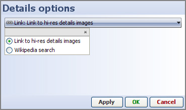 |
If you choose Popup details as the single record details display type, then click Edit individual details display options, you will see a three-tabbed dialog containing all the settings
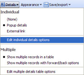 | General tab
Images tab
Fonts tab |
The General tab includes
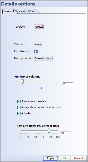 |
Template settings determine the layout of space in the details display window
Standard - Letterbox - Image only - No image - Vertical - Video -
|
Fields to show:
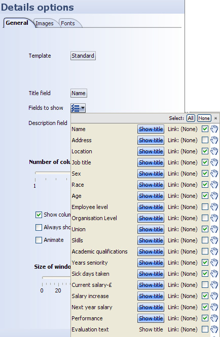 |
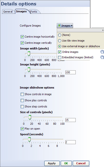 |
 |
(back to top) [94]
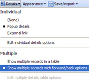
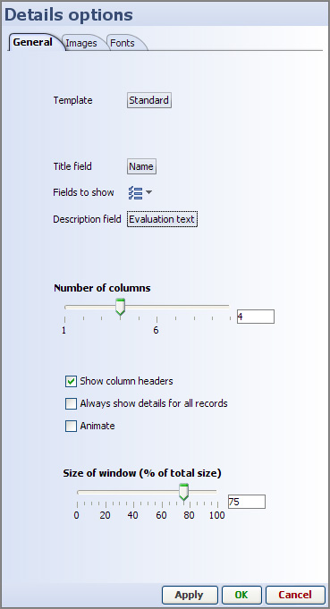
Templates are the same as those for individual record displays
Fields to show drop-down selector works the same as for individual record details display (see above)
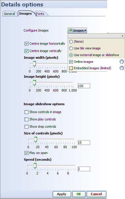
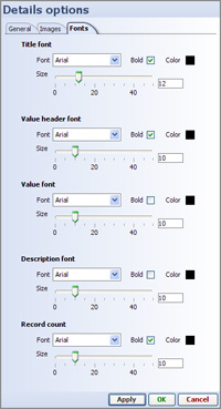
(back to top) [94]
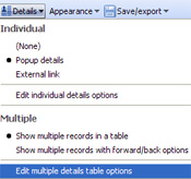
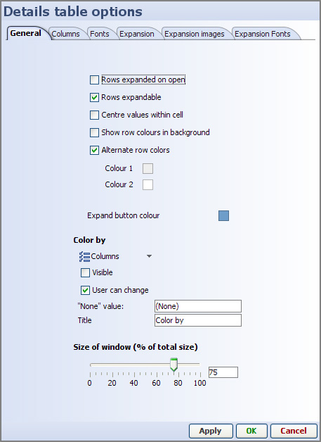
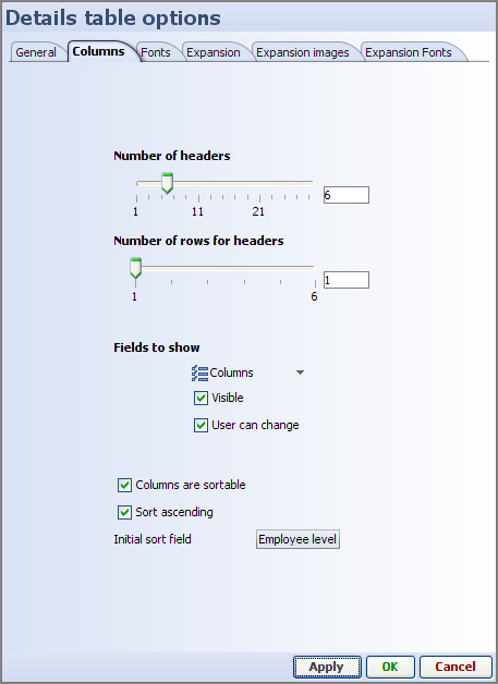
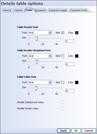
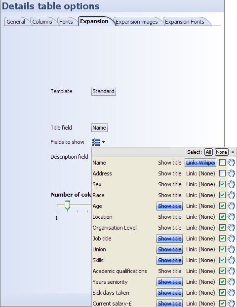
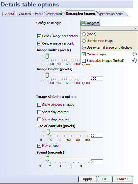
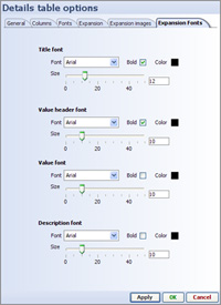
(back to top) [94]
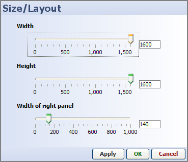 |
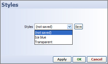 |  |
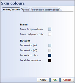 |  | 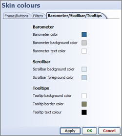 |
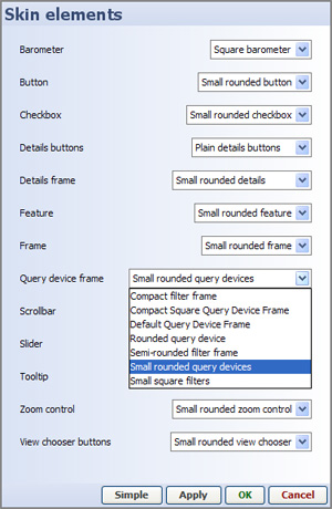 |

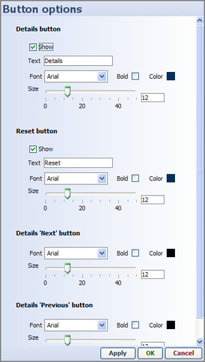
By default, the numbers or dates appear above the sliders. If you have short integer numbers, and mor horizontal space, you can un-tick the Text always above sliders option and the values will appear at the ends of the sliders. (not recommended for dates)
Relatively large data sets may not be able to synchronise the display with movement of the slider in real time. Use the Sliders filter on release option to de-couple movement of the slider from the up-date of the visualisation, improving the user experience.
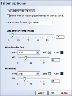
Sets colour options across all view types in the DataPlayer
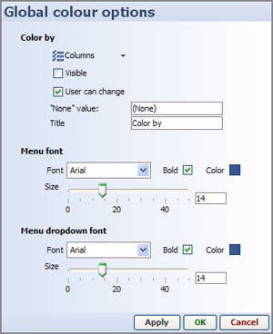
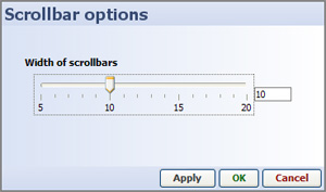
The column(s) to show as tooltips are currently a global Omniscope setting available from Settings > Tooltips (2.5)
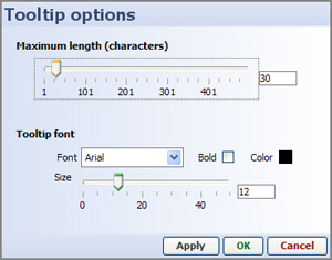
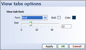
There are currently three options for exporting DataPlayers for display on the web:
If you choose this option, you will be asked to assign a password to the page/file and once your DataPlayer has been successfully uploaded, you will see the link to the page displaying your DataPlayer.
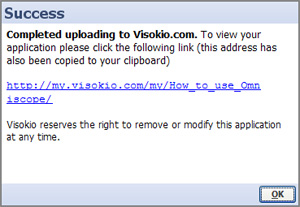 | You can use the resulting link in blogs and e-mails to display a blank web page with just your DataPlayer on it:
http://my.visokio.com/my/How_to_use_Omniscope/ [95]
You can update this online DataPlayer at any time by saving a new file to the same location with the exact same name (you will be asked for the password).
You cannot delete the page or the file, but you can upload a blank or re-directing version if you wish to display elsewhere and cannot recall the links you distributed. |
Choosing the Save for web option exports a blank .HTML file and an associated folder containing some 'helper' files and image folders.
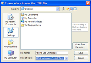 | Choose the name of the DataPlayer save for web file carefully, avoiding spaces and illegal characters, and using caution with upper and lower case naming. Omniscope will check for spaces and illegal characters, but preserve case in the names. Once you approve any changes to the name, Omniscope will save an .HTML page and an associated folder of files and images with the same name to the location you indicate. The blank HTML page can be used as a starting point for creating the page on which the DataPlayer will display, or the code between the <script> tags pasted into an existing display page. The folder of files should be uploaded to the web server preserving the name and the same relative position to the display page (immediate sub-directory). |
The exported Save for web folder contains any image folders (containing all the image files) used/referenced in the DataPlayer, the main .SWF DataPlayer file (with the extension _main.swf) and some helper files used to smooth the loading and display of the DataPlayer in site visitors' browsers.
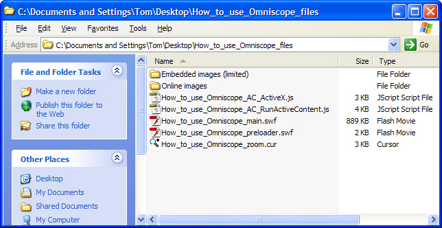
The easiest way of publishing the main SWF DataPlayer file on your intended display page is to use use your CMS to position the Flash file and generate the object tags. Alternatively, you can add hand-coded <object> tags following the model code below. Be sure to note the size of the DataPlayer and provide an appropriate space in the page.
<object classid="clsid:D27CDB6E-AE6D-11cf-96B8-444553540000"
codebase="http://download.macromedia.com/pub/shockwave/cabs/flash/swflash.cab#version=6,0,29,0"
width="750" height="290"><param name="movie"
value="/files/How_to_use_Omniscope_files/How_to_use_Omniscope_main.swf"
/><param name="quality" value="high" /><param name="menu" value="false" /><param name="wmode" value="" /><embed src="/files/How_to_use_Omniscope_files/How_to_use_Omniscope_main.swf"
wmode="" quality="high" menu="false" pluginspage="http://www.macromedia.com/go/getflashplayer [96]"
type="application/x-shockwave-flash" width="750" height="290"></embed></object>
ADVANCED: For advanced users, the blank HTML page exported together with the folder for upload contains the following code, reflecting the names you assigned when you saved the DataPlayer and when you created any associated image folders. If you wish to use scripts, you can paste this code into the various sections of your page.
<HTML><HEAD><script src="How_to_use_Omniscope_files/How_to_use_Omniscope_AC_RunActiveContent.js" type="text/javascript"></script><meta http-equiv=Content-Type content="text/html"; charset=ISO-8859-1"><TITLE>Visokio Omniscope - How_to_use_Omniscope</TITLE></HEAD><BODY align=center topmargin=0 leftmargin=0 marginheight=0 marginwidth=0><center><div style='margin: 10 10 10 10'><!-- using adobe javascript to pre-activate control - needs the How_to_use_Omniscope_files/How_to_use_Omniscope_AC_RunActiveContent.js script file --><script type="text/javascript"> AC_FL_RunContent( 'codebase','http://download.macromedia.com/pub/shockwave/cabs/flash/swflash.cab#version=6,0,47,0', 'width','750', 'height','290', 'id', 'preview', 'quality', 'high', 'bgcolor', '#FFFFFF', 'FlashVars', 'movieToLoad=How_to_use_Omniscope_files/How_to_use_Omniscope_main.swf', 'movie','How_to_use_Omniscope_files/How_to_use_Omniscope_preloader' );</script></div></center><!-- Javascript to get round IE "Click to activate and use control" --><script type="text/javascript" src="ieupdate.js"> theObjects = document.getElementsByTagName("object"); for (var i = 0; i < theObjects.length; i++) { theObjects[i].outerHTML = theObjects[i].outerHTML;}</script></BODY></HTML>If you have already published a DataPlayer and you wish to replace it with a more current .SWF containing refreshed data, or you wish to test the performance or other features, you can choose to export just the main .SWF file. Choose the name carefully, avoiding spaces and illegal characters, and using caution with upper and lower case naming. Omniscope will check for spaces and illegal characters, but preserve case in the names. If you are replacing an existing .SWF on the site, be sure to use the exact same name with the suffix 'main'. In the example above, the relative location and name of the file to be overwritten on your web server is shown following the code 'movieToLoad=
How_to_use_Omniscope_files/How_to_use_Omniscope_main.swf
Note: to display a standalone .SWF locally, you may need to associate the .SWF file extension with your browser.
Omniscope supports keyboard shortcuts to help you perform common tasks quickly. Because Omniscope is a Java rather than a Windows-only application, some shortcuts will differ from those used by Windows and/or Microsoft Office applications. For example, in Omniscope, Ctrl+F launches the Manage Fields wizard rather than Windows Find. Most Omniscope shortcuts are indicated on the command menus, but some, such as those used for Table View data entry and cell text editing do not have corresponding menus.
(Note: Apple Macs use the the Command key rather than Ctrl key + another key.)
Omniscope displays cells for editing in the Table View. To access the full body of text in a cell, double-click on the cell, or right-click and choose Edit this cell. The cell will expand to allow you to read many lines, but you cannot scroll down within a cell. The following keyboard shortcuts can be used to speed navigation and editing of cells containing many lines of text. These shortcuts are also very useful useful for copying values into cells down many rows or across many columns.
Alt+Return adds a return inside the text within a cell
Ctrl+End moves the cursor to the end/bottom of the text in the cell.
Ctrl+Home moves the cursor to the top of the text in the cell
Page Down moves the cursor a full page down the text
Page Up moves the cursor a full page up the text
Ctrl+A selects all the text in the cell,
Delete deletes all selected text
Backspace deletes selected cells or text
Ctrl+C copies the selected cells to the clipboard
Ctrl+V pastes the values in the clipboard to the selected cells (see warning on pasting in data below)
Ctrl+X removes the current values from the selected cells and stores them in the clipboard
Ctrl+Z undoes the previous edit
Ctrl+Y re-does the previous undone edit
Ctrl+; inserts the current date into the cell
Column headers are used to set sorting behaviour and cannot be used to select an entire column. To select most or all of a long column, hold the Shift key down and drag the right side scroll bar to the bottom of the target range. Then click on the last cell in the range and all intermediate cells will be selected and become targets for edits like copy and delete.
You can move data into or out of Omniscope using copy and paste (assuming the file owner has not locked the file).
WARNING: Be careful when pasting large, rectangular tables of values into the Omniscope via theTable View. If you specify a target paste range with more rows and columns than are contained in the data set you are copying, Omniscope will duplicate the records to fill the target space entirely. If you are not sure how many rows and columns you are importing via copy and paste, create a large number of new rows and columns and select only the single upper left-hand cell as the target paste range. This usually pastes the correct range. However, depending on the format/source of the incoming pasted data (web page tables, for example) all of the incoming values are sometimes pasted into the single upper left cell only. If this happens, then you must specify a rectangular target area exactly the correct size to receive the incoming pasted data. If you accidentally make the paste range too large, be sure to check for, and delete, any duplicated records.
F1 launches the Omniscope User Guide
F3 displays the About Visokio Omniscope screen with your license key and other important information about your installation
Ctrl+Alt+F1 opens the file-specific Help file configured by the file owner
Recent files: On opening, typing a number opens the file corresponding to that number in the recent file list
Ctrl+N opens new file
Ctrl+O opens existing file
Ctrl+S saves current file
Ctrl+Shift+S saves as new file
Ctrl+W closes the current file
Ctrl+E exports current (unaggregated) data set
Alt+F1 displays About screen summarising information about the file
Ctrl+F5 refreshes from the linked data source, if any
Ctrl+F6 refreshes Bloomberg-sourced fields with current Bloomberg values (Professional and Enterprise only)
F5 reloads data from source file
Ctrl+Shift+R recalculates all formulae
Ctrl+Alt+R recalculates a pre-defined subset of formulae (tab-specific)
Ctrl+F launches the Data > Manage Fields dialog
Ctrl+= adds record(s)
Ctrl+Shift+= adds field(s)
Ctrl+Delete deletes records(s)
Ctrl+D deselects all selected record(s)
Ctrl+Shift+D creates a new file for data management using File > New DataManager (2.6)
Ctrl+M executes a Move of selected record(s)
Ctrl+K executes a Keep of selected record(s)
Ctrl+R executes a Reset
Alt+Left Arrow History back
Alt+Right Arrow History forward
Ctrl+Q shows/hides the Side Bar
Ctrl+Tab inserts a tab in a multi-line editor (pressing tab alone will jump to the next element on the screen)
Ctrl+L launches the Styles dialog
Ctrl+Shift+B creates new blank Tab
Ctrl+Shift+N creates new Tab from current display
Ctrl+Shift+T creates new text slide Tab
Ctrl+Shift+I creates new image or PowerPoint slide Tab
Note: You can use the tab key to move from renaming a Tab, to the title editor, to the annotation editor
Alt+F1 displays Java tooltips
Ctrl+Home opens first Tab
Right arrow: opens next Tab
Left arrow: opens previous Tab
Escape cancels: open dialogs, mouse drag operations, current edits in text fields such as table cells, Tab titles and annotations
Enter commits edits in text fields, proceeds through wizard pages, closes or OKs dialogs
Ctrl+Enter commits multi-line text fields, such as Tab annotations
Alt+Enter inserts a line break
Ctrl+P prints the screen
Ctrl+Shift+P exports the current screen as an image
F9 resize to XGA (screen size 1024x768 pixels)
F11 toggle full screen mode. (Note: this function is experimental)
Ctrl+Shift+Alt+M launches memory diagnosis tool useful for optimising very large files for scaling and performance
Omniscope supports full Date & Time data typing, but unfortunately there are no international standards for formatting this type of data. Omniscope recognises most common Date & Time formats automatically on import, although Epoch/Unix formatted dates and times must be read in first as integer numbers (see below) [97]. If you create a new field (column) typed Date & Time, or if Omniscope does not initially recognise the formatting of your imported data, you may be asked to help Omniscope interpret the Date & Time formatting to facilitate the conversion, and also to specify how the imported values should be stored/displayed in Omniscope.
If Omniscope does not recognise a Date & Time column data formatting on import, it will probably initially data-type that column "Text", store the data as text values and display the column in the Table View with a white background, although sometimes the Date & Time formatting wizard will appear. Always confirm that all data which is supplied in the source data as Date & Time values has been successfully imported and typed Date & Time and therefore will be stored/displayed in Omniscope as full date/time values.
In both DataManager Field Organiser blocks or, if you have already loaded the data into the DataExplorer in memory data set, you can review and correct Date & Time data issues from the Main Toolbar: Data > Manage Fields data typing dialog:
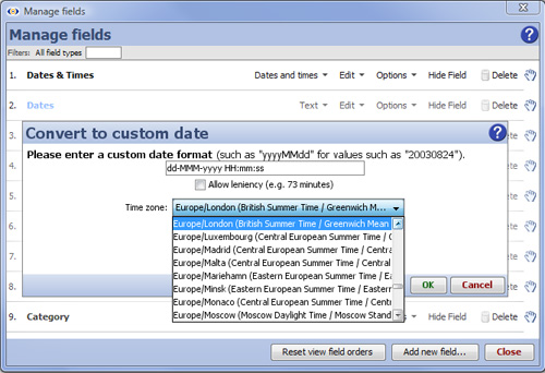
Use the Date & Time formatting wizard if Omniscope needs help detecting the format of existing data, or to change a column's Date & Time display format to another. If you specify the time zone, it is important to specify the time zone and daylight-savings time settings of the database server recording the data, which may be different from your own. It is possible for server clocks not respecting daylight savings time to record data inconsistent with the time zone setting you have selected. You must also respect leap year dates, and not enter non-existent dates. Invalid times or dates will NOT be coverted. (See below for further discussion of time zone and Daylight Savings Time-DST issues).
Spreadsheets often use two different columns to separate the calendar day-month-year Date from the clock hours:minutes:seconds Time. It is usually best to combine these two fields on import to Omniscope and store/display them within Omniscope as fully-formatted dates and times; dd/MM/yyyy HH:MM:ss. You can display any part of the Date/Time according to the display formatting you specify, but Omniscope's Java date/time arithmetic functions require the value to be stored fully-specified.
WARNING: When specifying date formats, make sure your data in the field/column is uniform. For example, if some cell values have Hours:Minutes:Seconds after the date, and you want to preserve this format in Omniscope, make sure that ALL cell values in that field have entries for Hours:Minutes:Seconds. If necessary, you can pad them out with all zero values like this: 00:00:00. Also, if you are using Date & Time fields as criteria for Omniscope merge file joins, make sure the fields are set to exactly the same format. If you intend to use AM/PM please make sure that your time is in 12 hour clock rather than in 24 hour clock format.
A date format is a user-specified sequence of case-sensitive characters describing the format of date/time values. For example, to show your dates as "16-Mar-2002" you would use the date format "dd-MMM-yyyy". You can use any punctuation, but letters must be in one of the valid patterns of characters listed below:
| Symbol | Meaning | Examples | Notes |
Dates: | |||
| yyyy | Year | 2002, 53, 1997, 500 BC | Literal year values, where "53" and "1066" will mean the years 53 and 1066 AD, and "200 BC" means the year 200 BC. |
| yy | Year | 02, 53, 97 | Two-digit years, with Y2K fix, where "53" and "10" will mean the years 1953 and 2010. Assumes any two-digit years fall within the last 80 years or next 20 years. |
| YYYY | Week year | 2012 | As per yyyy, except this is the "week year", i.e. the year of the current week-in-year, which is not always the same for a few days in the first and last weeks of the year. Only available in Omniscope installations based on Java 7, typically 2.8+. |
| w | Week | 1, 3, 52 | Week in year Warning: week of year yields different results in different locales, due to different regional settings for first-day-in-week. See Settings > Advanced file settings > Regional Settings (2.8+) |
| MMMM | Month | March, December | Full month name |
| MMM | Month | Mar, Dec | Abbreviated month name |
| MM | Month | 03, 12 | Two-digit month number, padded with zero |
| M | Month | 3, 12 | One- or two-digit month number, no padding |
| dd | Day of month | 03, 16 | Two-digit day in month, padded with zero |
| d | Day of month | 3, 16 | One- or two-digit day in month, no padding |
| EEEE | Weekday | Tuesday | Full name of day in week |
| EEE | Weekday | Tue | Abbreviated name of day in week |
Times: | |||
| aa | AM/PM | AM, PM | Use aa for the AM/PM marker |
| HH | Hour (24) | 00, 07, 15, 23 | Hour of day in 24-hour clock, from 0 to 23, padded with zero |
| H | Hour (24) | 0, 7, 15, 23 | Hour of day in 24-hour clock, from 0 to 23, not padded |
| hh | Hour (12) | 01, 07, 11, 12 | Hour of day in 12-hour clock, from 1 to 12, padded with zero |
| h | Hour (12) | 1, 7, 11, 12 | Hour of day in 12-hour clock, from 1 to 12, not padded |
| mm | Minutes | 00, 09, 23, 59 | Minutes past the hour, padded with zero |
| m | Minutes | 0, 9, 23, 59 | Minutes past the hour, not padded |
| ss | Seconds | 00, 09, 23, 59 | Seconds, padded with zero |
| s | Seconds | 0, 9, 23, 59 | Seconds, not padded |
| SSS | Milliseconds | 000, 009, 023, 595 | Milliseconds, padded with zero |
| S | Milliseconds | 0, 9, 23, 595 | Milliseconds, not padded |
| X | Timezone | -07, Z, +10 | ISO 8601 timezone, hours only (offset) or 'Z' for UTC |
| XX | Timezone | -0700, Z, +1000 | ISO 8601 timezone, hours and minutes (offset) or 'Z' for UTC |
| XXX | Timezone | -07:00, Z, +10:00 | ISO 8601 timezone, alternative ':' separated format, or 'Z' for UTC |
| dd-MM-yy | for values like: | 21-11-99 | meaning 21-11-1999 |
| yyyy.MM.dd | for values like: | 2001.07.04 | |
| yyyy.MM.dd HH:mm | for values like: | 2001.07.04 23:55 | |
| EEE h:mm a | for values like: | Sat 9:33 PM | |
| yyyy-MM-dd'T'HH:mm:ss.SSSZ | for values like: | 2001-07-04T12:08:56.235-0700 | |
| yyyy-MM-dd'T'HH:mm:ss.SSSXXX | for values like: | 2001-07-04T12:08:56.235-07:00 |
Databases record data using the time zone specified for that database. The database could be located anywhere in the world. In addition, the database may or may not reflect daylight savings time adjustments, even locally. If the data in the data set does not reflect daylight savings time, i.e. runs on GMT, and you select BST British summer time as a time zone for your data, Omniscope (and Java) will report invalid dates/times for some records. This occurs when daylight savings time adjustments 'skip over' one hour after midnight on specific dates. To fix this problem, you must isolate the offending times, and manually advance them by 1 hour.
The DATETOTEXT and TEXTTODATE functions allow you to specify time zones. Valid formats are as follows:
"GMT-08:00" or "GMT-8".
Epoch (or UNIX or POSIX) time is a system for describing points in time, defined as the number of (milli) seconds elapsed since midnight Coordinated Universal Time (UTC) of January 1, 1970, not counting leap seconds. Omniscope will import dates and times in this format if they are first read in as integer numbers. Once your data is imported as integer, in Data > Manage fields change the data type to Date & Time and select the option at the bottom Convert milliseconds since 1970 into dates. Omniscope uses milliseconds, so if your data is in seconds, multiply the values by 1000 using a formula column, then specify the Date & Time display format you wish to use.
The Data > Manage fields dialog is the central menu for accessing almost all commands that relate to adding, naming, showing or hiding, and removing fields (columns) from your data set. All of the fields (columns) in your data set will be visible here, even if you have hidden them in some or all views. Data typing, which tells Omniscope how to treat the values it finds in each field (column), can be centrally managed from this dialog.
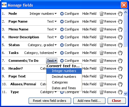
Note: Rename, Change Field type and Field options commands are also available from the Sidebar (right-click on filter device) and the Table View (right-click on column header).
For each field, the Field Type drop-down allows you to change the data type from the default assumptions made by Omniscope when the data was imported. Depending on your data source, Omniscope cannot always automatically determine the most suitable data type. The Field type drop-down shows the current data type, which may or may not be optimal for your analysis and reports. Omniscope classifies all data columns as either Integer numbers, Decimal numbers, Dates and Times, or Text. In addition, if the number of unique values in a column is less than about 250, Omniscope can treat each of the unique values in that column as a Category. It is important to use the most suitable data type for each column to get the best results.
Valid data types for values in each field (column) include:
Categories are a useful data type whenever a field (column) contains only a limited number (say 200-250) unique values, although the total number of records (rows) can be any number. Typical examples are a 'Sex' column, which usually contains only two unique values; 'Male' or 'Female', or list of distinct colours, such as 'red', 'orange' and 'green'. On data import, Omniscope will count the number of unique values, and for text columns will usually set the data type to be Category by default. Category fields also have the following options: Graded (the values are ordered and colour options shown with a continuous green to red scale, and Tokenized, meaning each cell can contain a delimited list of multiple values. See the discussion of Tokenized data [27].
Note: if you import data with a field containing a mixture of numbers and values such as "?", Omniscope will treat this as a Text or Category field. If you then convert the data type type to numbers, Omniscope will warn you before blanking out the "?" values.
Ordering and Resetting field orders- use the drag handles far right to re-order your columns from the default import order to the order you find most useful in the majority of the views. You can change this order view-by-view and in Reports Pages, but clicking on Reset field orders will return all views to this order, although hidden columns will remain hidden.
Add new field- creates a new, blank field in your file after the end of the list of existing fields. Enter the name, which must be unique, and click OK. Initially, the field will be a Category field, and all values will be blank (empty, also called null and shown in grey). Use the Field type drop-down to change the data typing to the desired field type (described above). Use the drag handles to move it into position between other fields, then click Reset field orders. This will display the new field in the Table View in the correct location. Note: New fields will remain hidden in Report Pages already configured. You must visit each Report Page and use the Columns/Fields to show option in each view to reveal the new field, then Commit the changes to make them persistent.
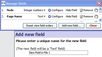
Click the Configure drop-down for each field to get other actions and configurations related to a field.
Rename field- often data sets imported from database tables rather than human-friendly views will have obscure field names which are not easy for those receiving your file to understand. Use this command to change the field (column) names in Omniscope...the data refresh process will not be affected. If you want to preserve the display of upper case acronyms, 'ISIN' rather than 'Isin'...be sure to tick the Preserve upper/lower case of field name option.
Change to formula field- converts a column from input values to calculated values according to a formula you specify. See Formulas & Variables.
Add field notes allows you to annotate a field; any text you enter here will appear in a tooltip whenever the mouse hovers over a Table View column header, or a Side Bar filter device. Use this to attribute the source of your data, clarify definitions, etc.
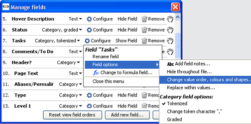
Hide throughout file- same as Hide Field, you will be asked explicitly if this applies to Report Pages already configured. If you do not want to hide the field in Report Pages where it is currently displayed, choose Skip Report Pages. Note: you can still reveal hidden fields in Side Bar filters using the Devices drop down.
Replace within values- same as the command available on the Edit menu
Edit value- Sometimes minor variations in spellings cause Omniscope to manage more distinct categories than actually exist. The Edit value command allows you to standardise spellings of potentially thousands of values in the data set in order to achieve the correct category listings.
Value order- this option applies to Category fields, for which you usually need to define a sorting order. By default, category values are sorted alphabetically. For many categories, alphabetical order is not meaningful. In the example below, a sequence of tasks in creating a web site have been dragged into a new order using the drag handles at far right. The Task values will now display and sort in this new, non-alphabetical order in all views. If we now choose to convert this field to a Graded Category, the new top and bottom values will define the colouring range (see below). Note: If you set a category sort order from top to bottom, and find that some views display the values in a sequence opposite to your preference, try reversing the sort order by dragging the Category values from bottom to top.
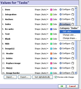
Import/Export- If you have a notepad file (.TXT) listing the values in correct business order, you can import the list and Omniscope will automatically arrange the sort order accordingly. You can also export a list showing the current sort order.
Sort alphabetically- returns the sort order to the default
For Category fields, if you don't like the colours chosen automatically for your Category values, or have specific colours you would like to use, click the square colour box next to the value you would like to change to display a Colour Chooser. This dialog enables you to select the colour associated with each Category value with great precision.
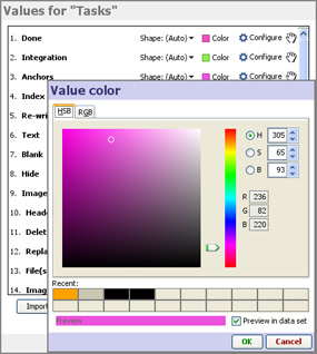
If your Category field is Graded (see above), you can't change Category values individually. Instead, you can choose start and end colours, and the values in between have a graded colour.
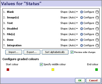
Date and Time, Integer and Decimal fields also allow you to change the gradation colours, with various options to achieve the best use of colour given any distribution of values within the field. You can specify the start and ending colours for the continuous range, and skew the colour spectrum by specifying the middle colour also.
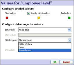 | 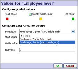 |
Numeric fields often have very skewed distributions due to extreme values, etc. and the resulting colour spectrum will be too uniform for most of the values. If you choose Fit to data behaviour, you can adjust for skewed data by selecting mean or skewed mean as a way of finding the 'middle' value for colouration purposes. If you have a more uniform distribution of values in your field, you may choose Fixed Range behaviour and specify Start, Middle and End values to achieve very precise colouring effects.
You can assign marker shapes to category values, such that different shapes are plotted on the Graph or Map view, depending on the value for the specified Shape field in each record.
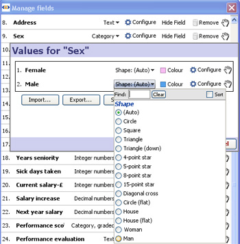
Sometimes, more than one value is associated with certain attributes of a record. For example, shoes can be available in more than one size, or you may have more than one image associated with with a house (or whatever). Shoe sizes and multiple images of a house are examples of many-to-one relationships. Omniscope handles these kinds of relationships using a 'Tokenised' data subtype for Text and Category fields (columns).
When you declare a Text or Category data type to be 'Tokenised,' it means each cell in a field can contain more than one value, i.e. multiple "tokens" separated by a character you decide. The default separator is a comma, but you can choose to use any character: a space to separate words, or an unusual character such as a " \ " backslash if you need to use commas within your values.
The example below (you can download a copy of this example file here [100]) is a sample shoe store data set. Each record (row) corresponds to a pair of shoes, and the 'Sizes available' field contains size numbers in stock (38, 39, 40, 41 etc.). The 'Sizes available' field has been typed a Category field since it contains only a few discrete values, the size numbers must be individually filterable (show me only my size) and the numbers treated as text, not numbers used for calculations.
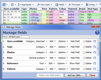 | Example: using Data > Manage fields > Configure > Field options, we can set the data sub-type of the 'Sizes available' Category field to be 'tokenised category' with the default comma separator dividing the values within the cells. We then check the data to ensure that each available shoe size is entered in the 'Size' column with a comma separator as shown in the Table View above. We can quickly check that all values have been entered correctly in the Sidebar query device for 'Size', because each size should appear separately. |
In the example below, the user has selected a specific shoe style. Notice that in the Chart View, the highlighting for a specific pair of shoes highlights the full range of sizes available. This behaviour is the same in all other views that display breakdowns of Tokenised Categories, such as the Pie and Tile Views.
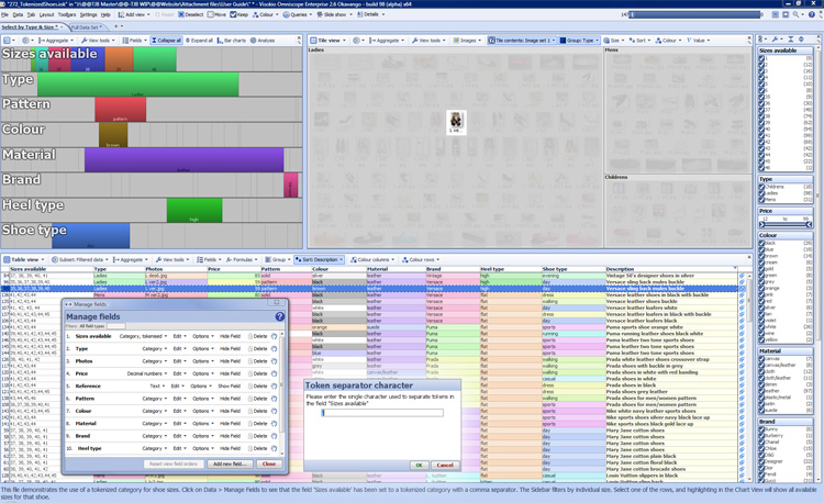
If there were multiple images for each pair of shoes, we would have done the same thing in the 'Photos' image references field (column), so that we could relate more than one image to each pair of shoes, and display the multiple images in the details display.
Note: See also examples of commonly-used formulae [101], or consult the Functions Guide [102] for documentation of all functions available for use in formulae.
Omniscope allows you to add formula fields, which are special fields (columns) whose values are calculated and re-calculated on opening/refresh according to the defined formula using inbuilt functions. Formulae combine references to other fields, mathematical expressions, a standard set of functions similar to spreadsheets such as Excel, and additional Omniscope-specific Subset functions which operate on evaluated subsets of your overall data set. Formulae in Omniscope are written in a similar sytax to spreadsheet formulae, using an interactive, visual editor and some easy-to-use variables for defining assumptions and sensitivity ranges. Subset functions do not exist in spreadsheets and therefore have their own syntax unique to Omniscope.
Formulas are composed and edited using Omniscope's powerful Omniscope Formula editor [103] which provides error feedback, preview of partial results and function assistance. Omniscope also allows you to define additional values called Variables [104], which are input assumptions, rather than values found within the fields (columns) of the data set. Variables have a single value, but are usually presented in a device allowing the user to change the value across a configurable range (see Add/Edit variables below). Variables are used for enabling multi-variate, dynamic sensitivity analyses and real-time modelling options that can be controlled by any user of the file.
This example below shows a formula for calculating staff salary increases based on performance scores using a conditional IF statement to test a field text value and apply the corresponding Variables:
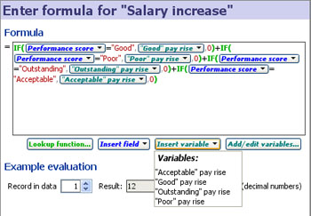 |  |
This example is taken from the embedded demo file File > Demos > Human resources, tab: Salary cost analysis. The data includes a column called 'Performance score' with 4 values; '"Acceptable", "Good", "Outstanding" and "Poor". The formula above uses nested IF functions (in green) and compares the value in the field'Performance score' (in blue), with typed in test values (enclosed in double quotes) reflecting the names of the Variables already defined, such as "Good" (in red). If the values match, i.e. an employee's value in the 'Performance score' column is "Good", then they will receive the pay rise defined by the Variable 'Good Pay rise'(since all the other IF comparisons will fail and the other parts of the expression will be zero). The Variable 'Good pay rise' has a default value (10) and a range. Each Variable defined also has an associated Side Bar device. If you reveal the Variables on the Side Bar, users of the file can perform real-time modelling and sensitivity analysis just by changing the assumed values using the sliders (see above right).
Unlike formulae in spreadsheets based on individual cell references, Omniscope formulae only contain field references, which are equivalent to saying "the cell in column X in the same row". You cannot define an Omniscope formula that depends on the value in a cell belonging to another record (row).
Formula fields can be added and defined using the Formula Editor accessible from the Main Toolbar using Data > Formulas and also from within the Table View using the Formulas button.
Use Data > Formulas > Add formula field to create a new field whose values calculated using a formula. You will be prompted to enter the name of the new field, before seeing the Formula editor [103] which you use to edit your formula.
 | 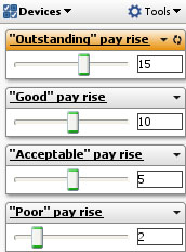 |
To edit an existing formula, choose Data > Formulas > Edit formula. You will first be prompted to choose the formula field.
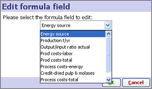
Alternatively, use the field menu to edit the formula for a given field. Field menus can be found by right-clicking the Table View column header, right-clicking the Sidebar filter device title, or through the Data> Manage Fields [31] window. The Formula Editor [103] will open showing your existing formula which can be edited as text.
If you already have a blank field with the correct name, right-click the column header in the Table View, or use the Edit option in Data > Manage fields [31]. From the menu, choose Change to formula field. Alternatively, use Data > Formulas > Convert existing field to use formula. If the field already has data in its cells, you will be warned, as these values will be replaced with the formula results. The Formula Editor [103] will open allowing you to enter the formula.
Variables [104] are values with ranges you define which are not contained in the data set, but are available to be used in Formula field calculations. Variables [104] can take on a range of values, and if you reveal the corresponding Side Bar device, you and users of your files can 'use Side Bar sliders a check-boxes to 'flex' the model assumptions, performing real-time, multi-variate simulations and sensitivity analysis, with all views and totals updating automatically. For more detail on defining, manipulating and using variables in formulas, see Defining Variables [104].
Omniscope automatically recalculates all formulas where necessary when any of their dependencies change. If you edit a value in a field, any formulas that refer to it will recalculate for the same record. Formulas that refer to the sum of the entire field will recalculate for all records. If you adjust a Variable, any formulas that refer to it will recalculate for all records. In short, Omniscope takes care of ensuring your formulas and data are always consistent.
Formulas that change over time (for example, those that use the RAND() function) are recalculated when you open the file. You can tell Omniscope to recalculate all your formulas by using Data > Formulas > Recalculate all values. Or, to recalculate a single field, use Data > Manage fields [31] > Edit > Recalculate values.
If you are working on a large and complex model, you may wish to disable automatic recalculation of formulas by deselecting Data > Formulas > Calculate automatically. This will make Omniscope perform faster when adding and deleting fields, for example. Be warned that any edits to formulas will not be recalculated until you manually use Recalculate [all] values. Any formula fields you add will appear blank until you trigger recalculation.
You can remove the formula for fields while retaining their data as static values using Data > Manage fields [31] > Edit > Change to static values (for a single field) or Data > Formulas > Convert all formulas to static values. The data will be unchanged, but will no longer be recalculated when you change variables or update your data. You can restore the formula by changing back to a formula field (see above).
If you want to remove the underlying formula altogether from the file, perhaps to keep your trade secrets, use the Convert and erase option in the dialog shown when converting to static values. Alternatively, in the File > Save as dialog, tick Convert formulas to static values to export a file with all formulas removed and erased, with only the formula results as static data.
Sometimes a formula can appear to be written correctly but may fail when evaluating certain records. One example is where you are dividing by a field in one of you formulas, and that field contains a zero.
When this happens, the Table view's Formula button will be highlighted in red/pink, and on clicking it, View last formula error will appear in the menu. Choose this item to open the formula editor for the field with the problem. The Example evaluation > Record in data spinner will be preconfigured to show the record with the problem, and the Errors section will show the error for that record.
It can also be useful to find out what fields a formula references, and conversely, what formulas a field is used in. Hover over a field anywhere in the application (such as in Data > Manage Fields [31]) to see a summary of that field's "References" (if it is a formula field) and "Referenced by" (if it is referenced by other formulas).
This section expands on the Formula Editior Omniscope documentation of functions available for use in formula fields to calculate values based on values in other columns. Most of the functions/syntax are the same as those used in spreadsheets like Excel, but there are also powerful Omniscope-specific SUBSET functions that perform operations on evaluated data subsets, both aggregated and disaggregated.
See also: Useful formulae [105] Guide to SUBSET functions [106] Deprecated functions [107] Additional functions in Javascript [108] Explore this list in Omniscope [109]
Function | Usage | Description |
| ABS | ABS(number) | Returns the absolute value of a number, a number without its sign. |
| ACOS | ACOS(number) | Returns the arccosine of a number, in radians in the range 0 to Pi. The arccosine is the angle whose cosine is Number. |
| ACOSH | ACOSH(number) | Returns the inverse hyberbolic cosine of a number. |
| ALLRECORDCOUNT (Omniscope 2.6+) |
ALLRECORDCOUNT() | Evaluates to the total number of records (rows) in all data, before any filtering or in-view aggregation has been applied. Not supported for dynamic evaluation in aggregated views. |
| AND | AND(logical1, logical2, ...) | Checks whether all arguments are TRUE, and returns TRUE if all arguments are TRUE. |
| ASIN | ASIN(number) | Returns the arcsine of a number in radians, in the range -Pi/2 to Pi/2. |
| ASINH | ASINH(number) | Returns the inverse hyperbolic sine of a number. |
| ATAN | ATAN(number) | Returns the arctangent of a number in radians, in the range -Pi/2 to Pi/2. |
| ATANH | ATANH(number) | Returns the inverse hyperbolic tangent of a number. |
| AVG | AVG(value1, value1, ...) | Returns the average (arithmetic mean) of its arguments. |
| BUCKET (Omniscope 2.6+) |
BUCKET(value, width, number_format_or_date_unit, date_format) In scripts: bucket(value, width, number_format_or_date_unit, date_format) |
Retrieves a range for a date or a number as a text value in the format "A to B". For numbers, use BUCKET(value, width, format); for dates use BUCKET(value, width, unit, format). In either case, "format" is optional. Date units can be one of: "year", "month", "week", "day", "hour", "minute", "second", "millisecond". Numeric examples: BUCKET(5, 10) = '0 to 10' BUCKET(0.08, 0.1) = '0 to 0.1' BUCKET(0.1, 0.1) = '0.1 to 0.2' BUCKET(0, 0.1) = '0 to 0.1' BUCKET(0.11, 0.1) = '0.1 to 0.2' BUCKET(1002, 10) = '1000 to 1010' BUCKET(10000, 11) = '9999 to 10010' Date examples where field1 is 10 Feb 2007 12:43: BUCKET([field1], 2, "hours") = '10 Feb 2007 12:00 to 10 Feb 2007 14:00' BUCKET([field1], 2, "hours", "HH:mm") = '12:00 to 14:00' BUCKET([field1], 2, "months", "dd MMM yyyy") = '01 Jan 2007 to 01 Mar 2007' BUCKET([field1], 2, "years", "dd MMM yyyy") = '01 Jan 2006 to 01 Mar 2008' BUCKET([field1], 12, "seconds", "HH:mm ss") = '12:43 00 to 12:43 12' |
| CATCH (Omniscope 2.7+) |
CATCH(sub_formula) | Suppresses all evaluation errors in the sub-formula. If an error occurs, results in null. |
| CELL (Omniscope 2.8+) |
CELL(field, record) In scripts: cell(field, record) |
Retrieves a cell value for a field using an absolute row number. The field must be a field name; see also FIELDNAME and FIELDCOUNT functions. |
| CHOOSE | CHOOSE(index_num, value1, value2, ...) | Chooses a value from a list of values, based on an index number (beginning at 1). |
| COMBIN | COMBIN(number, number_chosen) | Returns the number of combinations for a given number of items. |
| CONTAINS (Omniscope 2.6+) |
CONTAINS(text, sub_text) | Returns true if [sub_text] occurs anywhere within [text] (case insensitive). |
| CONVERT_LATLON_TO_OSGBX (Omniscope 2.7+) |
CONVERT_LATLON_TO_OSGBX(lat, lon) | Converts coordinates from the latitude value in WGS 84 (GPS lat/lon) to British National Grid (OSGB 36) X. |
| CONVERT_LATLON_TO_OSGBY (Omniscope 2.7+) |
CONVERT_LATLON_TO_OSGBY(lat, lon) | Converts coordinates from the latitude value in WGS 84 (GPS lat/lon) to British National Grid (OSGB 36) Y. |
| CONVERT_OSGB_TO_LAT (Omniscope 2.5+) |
CONVERT_OSGB_TO_LAT(osgbX, osgbY) | Converts coordinates from British National Grid (OSGB 36) to the latitude value in WGS 84 (GPS lat/lon). |
| CONVERT_OSGB_TO_LON (Omniscope 2.5+) |
CONVERT_OSGB_TO_LON(osgbX, osgbY) | Converts coordinates from British National Grid (OSGB 36) to the longitude value in WGS 84 (GPS lat/lon). |
| COS | COS(number) | Returns the cosine of an angle. |
| COSH | COSH(number) | Returns the hyperbolic cosine of a number. |
| CURRENTROW | CURRENTROW() | Evaluates to the row number of the record being evaluated. Numbering starts at 1. |
| DATE (Omniscope 2.7+) |
DATE(year, month, day, hour, minute, second, millisecond, timezone) In scripts: date(year, month, day, hour, minute, second, millisecond, timezone) |
Creates a date using numerical arguments. If omitted or null, the first value for each arguments is used. So, if year is null, year 1 is used. If month is null or omitted, January is used. Etc. BC dates are not supported. Illegal dates such as day 29 Feb on a non-leap year will be rolled over. Time zone is a text value in the format "GMT-8:00" or "PST"; if omitted, the local time zone is used. |
| DATEADD (Omniscope 2.5+) |
DATEADD(date, number, unit) In scripts: dateAdd(date, number, unit) |
Adds a specified number of a specified unit to a date. To subtract, use a negative number. Unit is optional; if not specified, "day" is assumed, otherwise it should be specified as: "year", "month", "week", "day", "hour", "minute", "second", "millisecond". |
| DATEDIFF | DATEDIFF(date1, date2, unit, approximate) In scripts: dateDiff(date1, date2, unit, approximate) |
Establishes the difference between two dates, as a decimal number of a specified unit (optional, default: "day"). If date2 is before date1, the result will be negative. E.g. the decimal number of weeks between two dates. Units should be specified as: "year", "month", "week", "day", "hour", "minute", "second", "millisecond". You can optionally choose approximate date difference for faster value calculation by specifying "true" for "approximate". Approximate date difference divides elapsed time between the two dates by the typical unit length (e.g. 30 days for days-in-month). |
| DATETOTEXT (Omniscope 2.6+ (for time zone argument)) |
DATETOTEXT(date_value, custom_format, time_zone) In scripts: dateToText(date_value, custom_format, time_zone) |
Converts a Date into text, optionally using a custom date format and time zone. For more information please click here [110]. |
| DATEUNIT (Omniscope 2.5+) |
DATEUNIT(date, unit) In scripts: dateUnit(date, unit) |
Retrieves a specified unit from a date as a numeric value. For example, the date "12 Feb 2006" has 12 as the "day" unit. Unit is optional; if not specified, "day" is assumed, otherwise it should be specified as: "year", "month", "week", "day", "hour", "minute", "second", "millisecond". NB. "days" is interpreted as "day of month", "weeks" as "week of year", and "hours" as "hour of day (24)". |
| DATEVALUE | DATEVALUE(text) | Converts a text string that represents a date to a date. For more options, see TEXTTODATE. |
| DECLARE (Omniscope 2.6+) |
DECLARE(name1, expression1, name2, expression2, name3, expression3..., sub_formula) | Declares one or more named values, each with a value expression, for repeated use in a sub-formula. The names must not clash with existing field or variable names, and must not be quoted. For more information, see DECLARE function [111]. |
| DEPENDENCIES (Omniscope 2.7 b414+) |
DEPENDENCIES(nested_formula, ref1, ref2, ref3...) | Provides a hint to Omniscope that the nested formula has references to other fields. Use this when you are building up field references in ways that Omniscope cannot automatically determine, such as via the SCRIPT function. Omniscope needs to know about all field references in a formula to ensure correct evaluation. Example: DEPENDENCIES(SCRIPT(` ... dataArray("MyField") ... refVal("MyOtherField") ... `), [MyField], [MyOtherField]) This tells Omniscope that the script has references to MyField and MyOtherField. |
| E | E() | Euler's number, e, also called the base of natural logarithms. |
| ENDSWITH (Omniscope 2.6+) |
ENDSWITH(text, sub_text) | Returns true if [sub_text] occurs in the end of [text] (case insensitive). |
| EQUIV (Omniscope 2.6+) |
EQUIV(value1, value2) | Returns true if [value1] is equivalent to [value2] (automatically converting between text, numbers and dates to attempt to find a match). |
| EXP | EXP(number) | Returns e raised to the power of a given number. |
| FACT | FACT(number) | Returns the factorial of a number, equal to 1*2*3*...*Number. |
| FIELDCOUNT (Omniscope 2.8+) |
FIELDCOUNT() In scripts: fieldCount() |
Returns the number of fields present. |
| FIELDFORMAT | FIELDFORMAT(value, field) | Converts any value into the text equivalent, using a field format. Warning: boolean values (true/false) will be translated using the current Language setting. Usage examples: FIELDFORMAT(424, [Field 1]) = "424.00" |
| FIELDNAME (Omniscope 2.8+) |
FIELDNAME(field_number) In scripts: fieldName(field_number) |
Looks up a field name by number, e.g. the 5th field. |
| FIELDNUMBER (Omniscope 2.8+) |
FIELDNUMBER(field_name) In scripts: fieldNumber(field_name) |
Looks up a field number by name (reverse of FIELDNAME). |
| FINDBETWEEN (Omniscope 2.7+) |
FINDBETWEEN(all, before, after) | Returns the first shortest matching text surrounded by [before] and [after], or null if not found. For example, FINDBETWEEN("apple apple orange plum pear apple banana pear", "apple", "pear") would return " orange plum " |
| FINDLASTBETWEEN (Omniscope 2.7+) |
FINDLASTBETWEEN(all, before, after) | Returns the last shortest matching text surrounded by [before] and [after], or null if not found. For example, FINDLASTBETWEEN("apple apple orange plum pear apple banana pear", "apple", "pear") would return " banana " |
| HTTPREDIRECT | HTTPREDIRECT(url) | Retrieves the HTTP redirect target for a URL, if the server provides one. |
| IF (Use of extended form requires Omniscope 2.5+) |
IF(logical_test, value_if_true, value_if_false) or IF(test1, value1, test2, value2, test3, value3..., else_value) | Checks whether a condition is met, and returns one value if TRUE, and another value if FALSE If the longer form is used, returns value1 if test1 is true, otherwise returns value2 if test2 is true, otherwise returns value3 if test3 is true..., otherwise returns else_value. For example: IF( [Coupon]<6, "less than 6", [Coupon]<7, "6 to 7", [Coupon]<8, "7 to 8", "8+" ) |
| INTCEIL | INTCEIL(number) | Rounds a number up to the nearest integer. |
| INTERSECTION (Omniscope 2.6+) |
INTERSECTION(subset1, subset2, ...) In scripts: intersection(subset1, subset2, ...) |
Returns the data subset which is the intersection of records for all data subset arguments. If a record is present in ALL supplied subsets, it will be present in the result. WARNING: this is an experimental function that has not been optimised for performance. Use alternative solutions such as extra formulas and the SUBSET function if performance is unacceptable. For more information, please visit SUBSET functions [106]. |
| INTFLOOR | INTFLOOR(number) | Rounds a number down to the nearest integer. |
| INTROUND | INTROUND(number) | Rounds a number to the nearest integer. |
| INVERSE (Omniscope 2.6+) |
INVERSE(subset) In scripts: inverse(subset) |
Inverts the set of included records of a data subset. All records included in the subset supplied will be excluded in the result, and vice versa. WARNING: this is an experimental function that has not been optimised for performance. Use alternative solutions such as extra formulas and the SUBSET function if performance is unacceptable. For more information, please visit SUBSET functions [106]. |
| ISO_COUNTRY_NAME (Omniscope 2.5+) |
ISO_COUNTRY_NAME(code, display_language) | Converts an ISO country code into readable form. The function uses two arguments: code. The ISO language code. This can be either a 2-letter code language code or a 3-letter code. display_language. Optional argument. The language of the function text result. This can be either a 2-letter code language code or a 3-letter code. |
| ISO_LANGUAGE_NAME (Omniscope 2.5+) |
ISO_LANGUAGE_NAME(code, show_country, display_language) | Converts an ISO language code into readable form. The function uses three arguments: code. The ISO language code. This can be either a 2-letter code language code, 2-letter language/country code or a 3-letter code. show_country. Optional argument. If this is set to true and a 2-letter language/country code is provided the country will be shown in brackets after the language. The default value is true. display_language. Optional argument. The language of the function text result. This can be either a 2-letter code language code or a 3-letter code. |
| LASTDAYOFMONTH (Omniscope 2.6+) |
LASTDAYOFMONTH(date_value) | Returns last day of month for a given date. Date value should include month and year value. |
| LAT_LON_DISTANCE (Omniscope 2.7+) |
LAT_LON_DISTANCE(lat1, lon1, lat2, lon2) | Returns the surface distance (in KM) from one latitude/longitude point to another. |
| LEFT | LEFT(text, num_chars) | Returns the specified number of characters from the start of a text string. |
| LEN | LEN(text) | Returns the number of characters in a text string. |
| LEVENSHTEIN (Omniscope 2.8+) |
LEVENSHTEIN(value1, value2) In scripts: levenshtein(value1, value2) |
Evaluates the Levenshtein distance [112] between two text values (case insensitive). |
| LG | LG(number) | Returns the base-2 logarithm of a number. |
| LN | LN(number) | Returns the natural logarithm of a number. |
| LOG | LOG(number, base) | Returns the logarithm of a number to the base you specify. |
| LOWER | LOWER(text) | Converts all letters in a text string to lowercase. |
| MAX | MAX(value1, value1, ...) | Returns the largest value in a set of values. |
| MID | MID(text, start_num, num_chars) | Returns the specified number of characters from the middle of a text string, given a starting position and length. |
| MIN | MIN(value1, value1, ...) | Returns the smallest number in a set of values. |
| MOD | MOD(number, divisor) | Returns the remainder after a number is divided by a divisor. |
| NORMDIST (Omniscope 2.8+) |
NORMDIST(x, mean, sdev, cumulative) In scripts: normDist(x, mean, sdev, cumulative) |
Gives the probability that a number falls at or below a given value of a normal distribution. X - is the value for which you want the distribution, mean (by default 0) - is the arithmetic mean of the distribution, sdev (by default 1) - is the standard deviation of the distribution, the value should be positive (>0) cumulative (by default TRUE) - is a logical value that determines the form of the function. If cumulative is TRUE, NORMDIST returns the cumulative distribution function; if FALSE, it returns the probability mass function. See also NORMSDIST: NORMDIST(x,mu,sigma,TRUE) = NORMSDIST((x - mu)/sigma). |
| NORMINV (Omniscope 2.8+) |
NORMINV(probability, mean, sdev) In scripts: normInv(probability, mean, sdev) |
It is the inverse of the NORMDIST function. It calculates the x variable given a probability. probability - is a probability corresponding to the normal distribution, the value should be in the range (0, 1), >0 and <1, mean (by default 0) - is the arithmetic mean of the distribution, sdev (by default 1) - is the standard deviation of the distribution, the value should be positive (>0). |
| NORMSDIST (Omniscope 2.8+) |
NORMSDIST(x, cumulative) In scripts: normSDist(x, cumulative) |
Gives the probability that a number falls at or below a given value of a standard normal distribution. X - is the value for which you want the distribution, cumulative (by default TRUE) - is a logical value that determines the form of the function. If cumulative is TRUE, NORMSDIST returns the cumulative distribution function; if FALSE, it returns the probability mass function. See also NORMDIST: NORMDIST(x,mu,sigma,TRUE) = NORMSDIST((x - mu)/sigma). |
| NORMSINV (Omniscope 2.8+) |
NORMSINV(probability) In scripts: normSInv(probability) |
It is the inverse of the NORMSDIST function. It calculates the x variable given a probability. probability - is a probability corresponding to the normal distribution, the value should be in the range (0, 1), >0 and <1. |
| NOT | NOT(logical) | Changes FALSE to TRUE, or TRUE to FALSE. |
| NOW | NOW() | Returns the current date/time. |
| NUM_OF_TOKENS | NUM_OF_TOKENS(text, token_separator) | Returns the number of tokens (split by a single character such as a comma) in a text value. |
| NUMVALUE | NUMVALUE(text) | Converts a text string that represents a number to a number. |
| OR | OR(logical1, logical2, ...) | Checks whether any arguments are TRUE, and returns TRUE or FALSE. Returns FALSE only if all arguments are FALSE. |
| PI | PI() | Returns the value of Pi, 3.141592653589793, accurate to over 15 digits. |
| POWER | POWER(number, power) | Returns the result of a number raised to a power. |
| PROPER | PROPER(text) | Converts a text string to proper case; the first letter in each word in uppercase, and all other letters to lowercase. |
| RAND | RAND() or RAND(seed) | Returns a random number greater than or equal to 0 and less than 1, evenly distributed. The result changes on every recalculation, unless a seed value (any number) is specified, in which case the number generated is always the same for a given seed. |
| RANK (Use of dataSubset argument requires Omniscope 2.5+) |
RANK(value, field, isAscending, includeNulls, dataSubset) | Returns the rank of a value within the field specified. This is the value position within the array of ordered field values. If isAscending parameter is not specified, FALSE or takes string "descending", the rank is against a descending order (higher values give better rank, with the highest number giving rank 1). If isAscending parameter is TRUE or takes string "ascending", the rank is against an ascending order. If the value is NULL, or not present in the list, NULL is returned, unless includeNulls is specified as true, in which case empty cells in the list will be considered. If dataSubset is specified, the RANK is calculated for a subset of the data which can be specified using the SUBSET function. Examples: RANK(10.1, [field1]) RANK(10.1, [field1], 1) RANK(10.1, [field1], true) RANK(10.1, [field1], "ascending") Valid argument combinations without data subset: RANK(field) (shorthand for RANK(field, field)) RANK(value, field) RANK(value, field, isAscending) RANK(value, field, isAscending, includeNulls) Valid argument combinations with data subset: RANK(value, field, dataSubset) RANK(value, field, isAscending, dataSubset) RANK(value, field, isAscending, includeNulls, dataSubset) For more information, please visit SUBSET functions [106]. |
| READRES | READRES(file_path_or_url, max_cache_age_seconds) | Reads the text contents from a file or URL. If the maximum cache age in seconds is not specified, it will be assumed to be 1 minute. Downloaded data will be cached for this period. Use -1 to disable caching. |
| RECORDCOUNT (Omniscope 2.5+) |
RECORDCOUNT(subset) In scripts: recordCount(subset) |
Evaluates to the number of records (rows) in the all data (if subset is not specified), or a subset (if subset is specified). The subset should be a data subset as evaluated using the SUBSET function. |
| REFVAL (Omniscope 2.6+) |
REFVAL(field_name) In scripts: refVal(field_name) |
Looks up the value of a field or variable by its name. The name can be dynamically determined, such as by concatenating text and/or using variables. |
| REPLACE | REPLACE(old_text, start_num, num_chars, new_text) | Replaces part of a text string with a different text string. |
| REPLACEREGEX (Omniscope 2.6+) |
REPLACEREGEX(text, regular_expression, replace_text, use_empty_if_no_match) | Replaces text matching a regular expression. In the replace text, use "$1" to refer to group 1 in the regular expression, and "$$" to mean a single dollar character. If use_empty_if_no_match (optional, default false) is true, and the expression does not match, results in null. For more information on regular expressions, see Regular expressions guide [113] |
| REPT | REPT(text, number_times) | Repeats text a given number of times. Use REPT to fill a cell with a number of instances of a text string. |
| RIGHT | RIGHT(text, num_chars) | Returns the specified number of characters from the end of a text string. |
| ROUND (Omniscope 2.8+) |
ROUND(number, num_digits) | Rounds a number to a specified number of digits. For example: ROUND(123.7825, 2) = 123.78 ROUND(123.456, 1) = 123.5 ROUND(123.456, -2) = 100); |
| ROWINDEXSUBSET (Omniscope 2.7+) |
ROWINDEXSUBSET(rowIndex, operator) In scripts: rowIndexSubset(rowIndex, operator) |
Results in a subset matching the row index(es) specified. Row indexes start from 1. Custom operator should be one of: "=", "<>", ">", ">=", "<", "<=" If not specified, "=" (equals) is used. |
| RUNNINGTOTAL (Omniscope 2.6+; 2.8+ for sortOrder) |
RUNNINGTOTAL(field, subset, sortOrder) | Evaluates to the running total in field for all data (if subset is not specified), or a subset (if subset is specified). The subset should be a data subset as evaluated using the SUBSET function. If sortOrder is true, values will sum in ascending order. If false, in descending order. If null or missing, in record order. |
| SCRIPT (Omniscope 2.6+; only with Java 6; some scripting functions require Omniscope 2.7+) |
SCRIPT(script, var1Name, var1Value, var2Name, var2Value, var3Name, var3Value..., timeout) | Executes a javascript expression. Requires Java 6, included with the full Omniscope installer. Supports core Javascript 1.5, but not browser-related objects. The script will be terminated after 10 seconds unless "timemout" is specified (in milliseconds). Note: you can use back-quotes (`) instead of normal quotes to quote your script, such as: `1 + 2`. Unlike with normal quotes, back-quoted text can contain any other character including backslash. For literal back-quotes, use two, e.g. SCRIPT(`var x = "Her name was ``Jane``";`) You must ensure you declare any dependencies (referenced fields inside your script) using the DEPENDENCIES function. For more information please click here [114]. |
| SEARCH | SEARCH(find_text, within_text, start_num) | Returns the number of the character at which a specific character or text string is first found, reading from left to right (not case-sensitive). The first character is numbered 1. Returns null if not found. |
| SEARCHREGEX | SEARCHREGEX(reg_expr, within_text, start_num) | Returns the number of the character at which a regular expression is first found, reading from left to right (not case-sensitive). The first character is numbered 1. Returns null if not found. For more information on regular expressions, see Regular expressions guide [113] |
| SIGN | SIGN(number) | Returns the sign of a number: 1 if the number is positive, zero if the number is zero, or -1 if the number is negative. |
| SIN | SIN(number) | Returns the sine of an angle. |
| SINH | SINH(number) | Returns the hyperbolic sine of a number. |
| SOUNDEX (Omniscope 2.8+) |
SOUNDEX(word) In scripts: soundex(word) |
Converts a text value containing a single word into its Soundex [115] phonetic code. |
| SQRT | SQRT(number) | Returns the square root of a number. |
| STARTSWITH (Omniscope 2.6+) |
STARTSWITH(text, sub_text) | Returns true if [sub_text] occurs in the beginning of [text] (case insensitive). |
| SUBSET (Omniscope 2.5+; Omniscope 2.6+ for custom operators) |
SUBSET(field, field_value, field_operator) In scripts: subset(field, field_value, field_operator) |
Evaluates to a subset of the data. Normally used only as an argument to another function. Either: (a) all records (if no arguments are specified); or (b) a current subset of records (if field is specified); or (c) another subset of records (if field and field_value are specified); or (d) another subset of records, using a custom operator (if all arguments are specified). Custom operator should be one of: "=", "<>", ">", ">=", "<", "<=", "contains" (2.8+), "does-not-contain" (2.8+), "starts-with" (2.8+), "ends-with" (2.8+) For more information, please visit SUBSET functions [106]. |
| SUBSET2 (Omniscope 2.5+; Omniscope 2.6+ for custom operators) |
SUBSET2(field_1, field_2, field_1_value, field_2_value, field_1_operator, field_2_operator) In scripts: subset2(field_1, field_2, field_1_value, field_2_value, field_1_operator, field_2_operator) |
Evaluates to a subset of the data. Normally used only as an argument to another function. Either: (a) a current subset of records (if field_N is specified); or (b) another subset of records (if field_N and field_N_value are specified); or (c) another subset of records, using a custom operator (if all arguments are specified). Custom operator should be one of: "=", "<>", ">", ">=", "<", "<=", "contains" (2.8+), "does-not-contain" (2.8+), "starts-with" (2.8+), "ends-with" (2.8+) For more information, please visit SUBSET functions [106]. Deprecated - please use the SUBSET and INTERSECTION functions instead. |
| SUBSET3 (Omniscope 2.5+; Omniscope 2.6+ for custom operators) |
SUBSET3(field_1, field_2, field_3, field_1_value, field_2_value, field_3_value, field_1_operator, field_2_operator, field_3_operator) In scripts: subset3(field_1, field_2, field_3, field_1_value, field_2_value, field_3_value, field_1_operator, field_2_operator, field_3_operator) |
Evaluates to a subset of the data. Normally used only as an argument to another function. Either: (a) a current subset of records (if field_N is specified); or (b) another subset of records (if field_N and field_N_value are specified); or (c) another subset of records, using a custom operator (if all arguments are specified). Custom operator should be one of: "=", "<>", ">", ">=", "<", "<=", "contains" (2.8+), "does-not-contain" (2.8+), "starts-with" (2.8+), "ends-with" (2.8+) For more information, please visit SUBSET functions [106]. Deprecated - please use the SUBSET and INTERSECTION functions instead. |
| SUBSET4 (Omniscope 2.5+; Omniscope 2.6+ for custom operators) |
SUBSET4(field_1, field_2, field_3, field_4, field_1_value, field_2_value, field_3_value, field_4_value, field_1_operator, field_2_operator, field_3_operator, field_4_operator) In scripts: subset4(field_1, field_2, field_3, field_4, field_1_value, field_2_value, field_3_value, field_4_value, field_1_operator, field_2_operator, field_3_operator, field_4_operator) |
Evaluates to a subset of the data. Normally used only as an argument to another function. Either: (a) a current subset of records (if field_N is specified); or (b) another subset of records (if field_N and field_N_value are specified); or (c) another subset of records, using a custom operator (if all arguments are specified). Custom operator should be one of: "=", "<>", ">", ">=", "<", "<=", "contains" (2.8+), "does-not-contain" (2.8+), "starts-with" (2.8+), "ends-with" (2.8+) For more information, please visit SUBSET functions [106]. Deprecated - please use the SUBSET and INTERSECTION functions instead. |
| SUBSET5 (Omniscope 2.5+; Omniscope 2.6+ for custom operators) |
SUBSET5(field_1, field_2, field_3, field_4, field_5, field_1_value, field_2_value, field_3_value, field_4_value, field_5_value, field_1_operator, field_2_operator, field_3_operator, field_4_operator, field_5_operator) In scripts: subset5(field_1, field_2, field_3, field_4, field_5, field_1_value, field_2_value, field_3_value, field_4_value, field_5_value, field_1_operator, field_2_operator, field_3_operator, field_4_operator, field_5_operator) |
Evaluates to a subset of the data. Normally used only as an argument to another function. Either: (a) a current subset of records (if field_N is specified); or (b) another subset of records (if field_N and field_N_value are specified); or (c) another subset of records, using a custom operator (if all arguments are specified). Custom operator should be one of: "=", "<>", ">", ">=", "<", "<=", "contains" (2.8+), "does-not-contain" (2.8+), "starts-with" (2.8+), "ends-with" (2.8+) For more information, please visit SUBSET functions [106]. Deprecated - please use the SUBSET and INTERSECTION functions instead. |
| SUBSET_EMPTYCOUNT (Omniscope 2.5+) |
SUBSET_EMPTYCOUNT(stat_field, subset) In scripts: subset_emptyCount(stat_field, subset) |
Calculates the statistical function [Number of empty values] of a field. Either: (a) for all records (if only field_name is specified); or (b) for a subset of data (if subset is specified). Use the SUBSET function to define a data subset. For more information, please visit SUBSET functions [106]. |
| SUBSET_FIRST (Omniscope 2.6+) |
SUBSET_FIRST(stat_field, subset) In scripts: subset_first(stat_field, subset) |
Calculates the statistical function [The first value (or null) in the original data order] of a field. Either: (a) for all records (if only field_name is specified); or (b) for a subset of data (if subset is specified). Use the SUBSET function to define a data subset. For more information, please visit SUBSET functions [106]. |
| SUBSET_FIRSTNONNULL (Omniscope 2.7+) |
SUBSET_FIRSTNONNULL(stat_field, subset) In scripts: subset_firstNonNull(stat_field, subset) |
Calculates the statistical function [The first non-null value in the original data order] of a field. Either: (a) for all records (if only field_name is specified); or (b) for a subset of data (if subset is specified). Use the SUBSET function to define a data subset. For more information, please visit SUBSET functions [106]. |
| SUBSET_LAST (Omniscope 2.6+) |
SUBSET_LAST(stat_field, subset) In scripts: subset_last(stat_field, subset) |
Calculates the statistical function [The last value (or null) in the original data order] of a field. Either: (a) for all records (if only field_name is specified); or (b) for a subset of data (if subset is specified). Use the SUBSET function to define a data subset. For more information, please visit SUBSET functions [106]. |
| SUBSET_LASTNONNULL (Omniscope 2.7+) |
SUBSET_LASTNONNULL(stat_field, subset) In scripts: subset_lastNonNull(stat_field, subset) |
Calculates the statistical function [The last non-null value in the original data order] of a field. Either: (a) for all records (if only field_name is specified); or (b) for a subset of data (if subset is specified). Use the SUBSET function to define a data subset. For more information, please visit SUBSET functions [106]. |
| SUBSET_MAX (Omniscope 2.5+) |
SUBSET_MAX(stat_field, subset) In scripts: subset_max(stat_field, subset) |
Calculates the statistical function [Maximum value (highest or last)] of a field. Either: (a) for all records (if only field_name is specified); or (b) for a subset of data (if subset is specified). Use the SUBSET function to define a data subset. For more information, please visit SUBSET functions [106]. |
| SUBSET_MEAN (Omniscope 2.5+) |
SUBSET_MEAN(stat_field, subset) In scripts: subset_mean(stat_field, subset) |
Calculates the statistical function [Mean (average) of values] of a field. Either: (a) for all records (if only field_name is specified); or (b) for a subset of data (if subset is specified). Use the SUBSET function to define a data subset. For more information, please visit SUBSET functions [106]. |
| SUBSET_MEDIAN (Omniscope 2.5+) |
SUBSET_MEDIAN(stat_field, subset) In scripts: subset_median(stat_field, subset) |
Calculates the statistical function [Median (middle) of values] of a field. Either: (a) for all records (if only field_name is specified); or (b) for a subset of data (if subset is specified). Use the SUBSET function to define a data subset. For more information, please visit SUBSET functions [106]. |
| SUBSET_MIN (Omniscope 2.5+) |
SUBSET_MIN(stat_field, subset) In scripts: subset_min(stat_field, subset) |
Calculates the statistical function [Minimum value (lowest or first)] of a field. Either: (a) for all records (if only field_name is specified); or (b) for a subset of data (if subset is specified). Use the SUBSET function to define a data subset. For more information, please visit SUBSET functions [106]. |
| SUBSET_MODE (Omniscope 2.5+) |
SUBSET_MODE(stat_field, subset) In scripts: subset_mode(stat_field, subset) |
Calculates the statistical function [Most common value (first if multimodal)] of a field. Either: (a) for all records (if only field_name is specified); or (b) for a subset of data (if subset is specified). Use the SUBSET function to define a data subset. For more information, please visit SUBSET functions [106]. |
| SUBSET_NONEMPTYCOUNT (Omniscope 2.5+) |
SUBSET_NONEMPTYCOUNT(stat_field, subset) In scripts: subset_nonEmptyCount(stat_field, subset) |
Calculates the statistical function [Number of non-empty values] of a field. Either: (a) for all records (if only field_name is specified); or (b) for a subset of data (if subset is specified). Use the SUBSET function to define a data subset. For more information, please visit SUBSET functions [106]. |
| SUBSET_PRODUCT (Omniscope 2.8+) |
SUBSET_PRODUCT(stat_field, subset) In scripts: subset_product(stat_field, subset) |
Calculates the statistical function [Product of values] of a field. Either: (a) for all records (if only field_name is specified); or (b) for a subset of data (if subset is specified). Use the SUBSET function to define a data subset. For more information, please visit SUBSET functions [106]. |
| SUBSET_RANGE (Omniscope 2.5+) |
SUBSET_RANGE(stat_field, subset) In scripts: subset_range(stat_field, subset) |
Calculates the statistical function [Range of values (maximum minus minimum)] of a field. Either: (a) for all records (if only field_name is specified); or (b) for a subset of data (if subset is specified). Use the SUBSET function to define a data subset. For more information, please visit SUBSET functions [106]. |
| SUBSET_SINGLETON (Omniscope 2.5+) |
SUBSET_SINGLETON(stat_field, subset) In scripts: subset_singleton(stat_field, subset) |
Calculates the statistical function [The single value, if there is one] of a field. Either: (a) for all records (if only field_name is specified); or (b) for a subset of data (if subset is specified). Use the SUBSET function to define a data subset. For more information, please visit SUBSET functions [106]. |
| SUBSET_STDDEV (Omniscope 2.5+) |
SUBSET_STDDEV(stat_field, subset) In scripts: subset_stdDev(stat_field, subset) |
Calculates the statistical function [Standard deviation of values from the mean] of a field. Either: (a) for all records (if only field_name is specified); or (b) for a subset of data (if subset is specified). Use the SUBSET function to define a data subset. For more information, please visit SUBSET functions [106]. |
| SUBSET_SUM (Omniscope 2.5+) |
SUBSET_SUM(stat_field, subset) In scripts: subset_sum(stat_field, subset) |
Calculates the statistical function [Sum (total) of values] of a field. Either: (a) for all records (if only field_name is specified); or (b) for a subset of data (if subset is specified). Use the SUBSET function to define a data subset. For more information, please visit SUBSET functions [106]. |
| SUBSET_UNIQUECOUNT (Omniscope 2.5+) |
SUBSET_UNIQUECOUNT(stat_field, subset) In scripts: subset_uniqueCount(stat_field, subset) |
Calculates the statistical function [Number of unique non-empty values] of a field. Either: (a) for all records (if only field_name is specified); or (b) for a subset of data (if subset is specified). Use the SUBSET function to define a data subset. For more information, please visit SUBSET functions [106]. |
| SUBSET_UNIQUESLIST (Omniscope 2.5+) |
SUBSET_UNIQUESLIST(stat_field, subset) In scripts: subset_uniquesList(stat_field, subset) |
Calculates the statistical function [A comma-separated list of all unique values] of a field. Either: (a) for all records (if only field_name is specified); or (b) for a subset of data (if subset is specified). Use the SUBSET function to define a data subset. For more information, please visit SUBSET functions [106]. |
| SUM | SUM(number1, number2, ...) | Adds all the arguments. |
| TAN | TAN(number) | Returns the tangent of an angle. |
| TANH | TANH(number) | Returns the hyperbolic tangent of a number. |
| TEXT_LINE_COUNT | TEXT_LINE_COUNT(text) | Returns the number of lines (split by line-break) in a text value. |
| TEXTTODATE | TEXTTODATE(text_value, custom_format, lenient, time_zone) In scripts: textToDate(text_value, custom_format, lenient, time_zone) |
Converts text into a date. If custom_format is specified, this is a custom date format pattern such as "dd/MM/yyyy HH:mm:ss". If not specified, the default format for the current data locale will be used. If lenient is omitted or is true, this controls whether non-existent dates are permitted, such as 29 February on a non-leap-year (corrected to 1 March). If time zone value is specified, this controls how Omniscope interprets time values. If not specified, the text will be assumed to be a date/time from the same time zone as the system. For more information on date and time formats please click here [110]. |
| TEXTVALUE | TEXTVALUE(value, pattern) In scripts: textValue(value, pattern) |
Converts any value into the text equivalent, optionally using a format pattern. The format pattern (which must be quoted text) defines how numbers or dates are formatted. Warning: boolean values (true/false) will be translated using the current Language setting. Usage examples: TEXTVALUE(424) = "424" TEXTVALUE(123456.789 , "$###,###.###") = "$123,456.789" TEXTVALUE(DATEVALUE("02/06/2009") , "yyyy.MMMM.dd") = "2009.June.02" For more information on date and time formats please click here [110]. For more information on number formats please click here [116]. |
| TODAY (Omniscope 2.5+) |
TODAY() | Returns the current date. |
| TRENDVALUE (Omniscope 2.8+) |
TRENDVALUE(xField, yField, subset, xValue) In scripts: trendValue(xField, yField, subset, xValue) |
Evaluates the linear trend for X and Y fields, then evaluates the Y value for X value specified. If 'xValue' is omitted, uses the current record's X value. Used to determine the Y coordinate in a best-fit line showing the trend of two fields. If 'subset' is omitted, the full dataset is used. |
| TRIM | TRIM(text) | Removes all spaces from a text string except for single spaces between words. |
| TYPEOF (Omniscope 2.6+) |
TYPEOF(arg) | Returns the type of the argument. |
| TZCORRECT (Omniscope 2.8+) |
TZCORRECT(date, input_timezone, output_timezone) In scripts: tzCorrect(date, input_timezone, output_timezone) |
Corrects dates in the wrong timezone. Converts from one timezone to another, preserving the same logical local time in each timezone. Observes the current and historical rules for time zone offset and daylight saving according to the Olson time zone database. For example, if your data was recorded as 9am in time zone X, but it should have been recorded as 9am in time zone Y, you would use: TZCORRECT(date, X, Y) If either time zone is missing, your file's time zone will be used, as configured in the Regional Settings dialog, which defaults to your local system time zone. |
| TZDEFAULT (Omniscope 2.8+) |
TZDEFAULT() In scripts: tzDefault() |
Returns the Olson ID for the default time zone for this file, as configured in the Regional Settings dialog, which defaults to your local system time zone. |
| TZOFFSET (Omniscope 2.8+) |
TZOFFSET(time_zone, date) In scripts: tzOffset(time_zone, date) |
Returns the UTC offset, in milliseconds, for the time zone specified. If time_zone is not supplied, your file's time zone will be used, as configured in the Regional Settings dialog, which defaults to your local system time zone. If date is specified, returns the offset for that date/time, observing the current and historical behaviour and daylight saving rules. If not specified, returns the current offset from UTC for standard time in that time zone (i.e. without daylight saving). |
| UNION (Omniscope 2.6+) |
UNION(subset1, subset2, ...) In scripts: union(subset1, subset2, ...) |
Returns the data subset which is the union of records for all data subset arguments. If a record is present in ANY supplied subset, it will be present in the result. WARNING: this is an experimental function that has not been optimised for performance. Use alternative solutions such as extra formulas and the SUBSET function if performance is unacceptable. For more information, please visit SUBSET functions [106]. |
| UNIX_MILLISECONDS_TO_DATE (Omniscope 3.0+) |
UNIX_MILLISECONDS_TO_DATE(unixtime) In scripts: unixMillisecondsToDate(unixtime) |
Converts a number of milliseconds since unix epoch (00:00 1 January 1970 UTC) to a date. |
| UNIX_SECONDS_TO_DATE (Omniscope 3.0+) |
UNIX_SECONDS_TO_DATE(unixtime) In scripts: unixSecondsToDate(unixtime) |
Converts a number of seconds since unix epoch (00:00 1 January 1970 UTC) to a date. |
| UPPER | UPPER(text) | Converts all letters in a text string to uppercase. |
| VALUE | VALUE(text) | Converts a text string that represents a number to a number, or date text into a date, where possible, otherwise resulting in a text value. |
| XPATH (Omniscope 2.6+) |
XPATH(xml_data, xpath_expression) | Executes an XPath expression against an XML document. To obtain XML data, see the READRES function. For more information on XPath, see XPath guide [117] |
Scripting format is shown for functions available in Content View scripts, etc., from 2.7. More detail [118].
Below are some examples of formulae useful for calculating commonly-used fields:
Note: You can type function names or pick from the list; text strings in quotes should be entered literally; field names in [ ] should be input using the [Insert field ] tool in the Formula Editor. [103] Given that every Omniscope file is potentially a template file that will be refreshed with future data from the linked source(s), it is good practise to write formulae that always test for null or zero values that may appear in future refreshes, potentially creating errors in formulae.
To create a new column categorising values in a source column according to user-defined upper and lower limits:
=IF([SourceColumn]=null,null,IF[SourceColumn]<50,"0-50",IF[SourceColumn]<500,"50-500",">500"))
In this example, each value in [SourceColumn] is evaluated first to see if the value is null, otherwise it is placed in one of three 'bucketing' categories: 0-50, 50-500, or >500
Dates of payments and other events sometimes need to be categorised by fiscal rather than calendar year. One way to do this is to use the following formula, which can be extended to any number of years:
=IF([Date]=null,null,IF(DATEDIFF(DATEVALUE("1 Oct 2001"),[Date],"day")<366,"FY2002",IF(DATEDIFF(DATEVALUE("1 Oct 2002"),[Date],"day")<366,"FY2003","Out of range")))
In this example, the company's fiscal year runs from October, and the formula column Fiscal Year will be populated with null, FY2002, FY2003, or "out of range" depending on the value in the [Date] field.
Date fields can be translated into various transformations and sub-components by specifying a custom output date format [119] as the second argument in the DATETOTEXT function. For example:
=DATETOTEXT([DateField],"w") ...this formula evaluates [DateField] and returns the corresponding week number.
=DATETOTEXT([DateField],"EEEE") ...this formula evaluates [DateField] and returns the corresponding day of the week
An especially useful version of this is used to create duplicate date columns typed as Categories which sort:
=DATETOTEXT([DateField],"yyyy-MM-dd")
You can then Pane views by this categorised date, and use category tick-boxes with the dates naturally in the correct sort order.
Often it is useful to categorise records based on their rank in a certain column, i.e. a "Top 10" category. The formula below assigns the category value "Top 10" to any record whose non-null value in column B is ranked 10 or less:
=IF(AND([B] != null, RANK([B])<=10), "Top 10", null)
Note: '!=' means 'not equal'. Having creating the dynamically-evaluated Category value "Top 10", you can then filter on it and define a Top 10 Named Query data subset such that other views can be set to display only the current Top 10 list of records.
Example File: Ranking Top 10 and Bottom 5 [120] ; Example File: Ranking Data Subsets [121]
Using a Variable to define the threshold, you can flag Values which are outside a user-selectable upper-lower tolerance range:
=IF(OR([Value]<(-1*{Threshold variable}),[Value]>{Threshold variable}),"Flagged","Not Flagged")
Before writing the formula, you must define the Threshold Variable, its min, max and default values
Counting the number of times a particular value appears in a column:
=DATASET_NONEMPTYCOUNT("Column Name","Column Name", [Insert field-Column Name])
The first free text input "Column Name" specifies the column, the second the non-empty and the last is an [Insert Field] of the field 'Column Name' to pick up the values. This admittedly obscure syntax will return for each row the total number of times the value in the row appears in that same column in the entire data set.
Sometimes incoming data sets have null values and for aggregation purposes these values need to be converted to zeros:
=SUM([Field containing nulls])
This formula reads the values in any number of fields, and if they are all null, will return a zero for that row
Unlike spreadsheets, Omniscope formulae do not reference cells or rows directly, but common calculations involving periodic differences over time can be done using Date functions and Subset functions, as illustrated by the attached file which calculates price changes on a security which is only traded on weekdays:
Example file - Calculating Periodic Changes over Time [122]
This page describes the latest functionality available in Omniscope 2.6 b607 and later. If you are using 2.5 or an earlier version of 2.6, please see the older guide [123].
SUBSET functions are unique to Omniscope and are broken down into two sub-classes of functions which work together:
Note: these replace the previous, now deprecated DATASET_... functions as they are more flexible and efficient. Other functions other than SUBSET_MEAN/SUM/etc. also use SUBSET 'clauses' such as RANK.
The new INTERSECTION, UNION and INVERSE functions are classed as experimental because they have not been optimised for performance. If you find they perform too poorly for your data size, please continue to use the older SUBSET2 etc. functions documented here [123]. Performance improvements are scheduled for 2.7.
| If you wanted to find: | The sum of Sales Volume for the current country |
which could be rewritten as: | Sum of Sales Volume in subset: [all records with the same Country as the record being evaluated] |
you would use the formula: | SUBSET_SUM([Sales Volume], SUBSET([Country])) |
SUBSET [124] 'clauses' results in a data subset for use in other functions (such as SUBSET_MEAN or RANK). You would not normally use the result of SUBSET 'clause' as the end result of the entire formula, since you cannot display the definition of the subset defined as a data table inside a cell.
SUBSET [124] 'clauses' are used to identify records by one constraint (e.g. Month is "February"). To identify records by multiple constraints, or use more complex logic, combine SUBSET [124] with INTERSECTION [125], UNION [126] and INVERSE [127] (e.g. All of records in [Month is "February"] and [Client is "Acme Bank"]).
| SUBSET() | The entire dataset |
| SUBSET([Month]) | Data subset with the same Month field value as the record being evaluated |
| SUBSET([Month], "February") | Data subset with the Month field value 'February' |
SUBSET([Quantity], 5) | Data subset where the field/column Quantity value equals 5 |
| SUBSET([Quantity], 5, "<") SUBSET([Quantity], 5, "<=") SUBSET([Quantity], 5, ">") SUBSET([Quantity], 5, ">=") SUBSET([Quantity], 5, "=") SUBSET([Quantity], 5, "<>") | Data subsets where the field/column Quantity value is less than, less than/equal, greater than, greater than/equal, equal, not equal to the value 5 (respectively). Use of the "operator" inequality options requires Omniscope 2.6+. |
SUBSET([Surname], "Mac", "starts-with") | Data subsets where the field Surname begins with "Mac" such as "MacDonald", or contains "-" such as a double-barrelled name, etc. (2.8+) |
INTERSECTION( SUBSET([Month]), SUBSET([Client]) | Data subset with the same Month and Client field values as the record being evaluated |
INTERSECTION( SUBSET([Month], "February" ),
SUBSET([Client], "Acme Bank" ) )
| Data subset with the Month and Client field values 'February' and 'Acme Bank' |
INTERSECTION( SUBSET([Month] ),
SUBSET([ Client ]),
SUBSET([Country] ) | Data subset with the same Month, Client and Country field values as the record being evaluated
|
INTERSECTION( SUBSET([Month],
), "February"
SUBSET([ Client ],Acme Bank " " ),
SUBSET([Country], "UK" ) | Data subset with the Month, Client and Country field values 'February', 'Acme Bank' and 'UK' |
INTERSECTION( SUBSET([Month], "February", "=" ),
SUBSET([ Client ],Acme Bank " " ,"= " ),
SUBSET([Quantity], 5, ">=" ) | Data subset where the Month and Client field values are 'February' and 'Acme Bank', and the Quantity field values are greater than or equal to 5. |
SUBSET_... functions (such as SUBSET_MEAN [128]) accept a field for the statistical function and an optional data subset 'clause' to restrict the record set.
SUBSET_MEAN([Price]) | The mean of the Price field, for all records |
| SUBSET_SUM([Price], SUBSET([Month])) | The sum of the Price field, for the data subset with the same Month field value as the record being evaluated |
| SUBSET_MODE([Currency], SUBSET([Month], "February")) | The most common Currency field value, for the data subset with the Month field value 'February' |
This example shows a table of data containing Traders and their Sales Volume by Country. We want to find out the total Sales Volume for each Trader.
Country | Trader | Sales Volume | Formula field |
| UK | John Swires | 10,000 | 60,000 |
| France | John Swires | 15,000 | 60,000 |
| USA | John Swires | 35,000 | 60,000 |
| UK | Anne Campbell | 7,000 | 21,000 |
| Japan | Anne Campbell | 14,000 | 21,000 |
The field "Formula field" above is defined with the formula:
SUBSET_SUM([Sales Volume], SUBSET([Trader]))
Broken down, this means:
SUBSET([Trader]) The records with the same Trader value as the record being evaluated
SUBSET_SUM([Sales Volume], subset) The sum of Sales Volume for those records
When Omniscope evaluates the first cell (60,000) in "Formula field":
SUBSET([Trader]) evaluates to all records with Trader "John Swires" (i.e. the first 3 records).
SUBSET_SUM([Sales Volume], subset) evaluates to 60,000 (10,000 + 15,000 + 35,000).
This example involves a table of data containing multiple quotes for multiple parts to multiple clients in multiple currencies. We want to find the lowest Quote in "USD" for each combination of Part and Customer.
Customer | Currency | Part | Quote | Min USD Quote | ||
Alpha | GBP | widget | 8 |
|
| 12 |
Beta | USD | gromett | 10 |
|
| 10 |
Gamma | Yen | nubbin | 50 |
|
| 6 |
Alpha | USD | widget | 12 |
|
| 12 |
Gamma | USD | widget | 9 |
|
| 9 |
Beta | Euro | gromett | 11 |
|
| 10 |
| Alpha | Yen | nubbin | 52 | 6 | ||
| Beta | USD | nubbin | 5 | 5 | ||
| Gamma | USD | gromett | 7 | 7 | ||
| Alpha | USD | nubbin | 6 | 6 | ||
| Gamma | USD | nubbin | 6 | 6 |
The formula field [Min USD Quote] above can be defined with the following formula:
SUBSET_MIN([Quote], INTERSECTION(SUBSET([Customer]), SUBSET([Currency], "USD"),
SUBSET([Part]))
Broken down, this formula means:
SUBSET_MIN( [Quote], find the lowest quotation in the column for the following subsets:
INTERSECTION(SUBSET([Customer]), SUBSET([Currency], "USD"), SUBSET([Part])) = all combinations of 'Customer' and 'Part' where Currency="USD"
The RANK function works much like the Excel RANK function, and allows you to infer the RANK of a value within a set of values. In Omniscope, the value can be any literal value or the value of a referenced field. The set of values must be all values within a named field, either for all records, or for a data subset.
Examples for the above Customer/Currency/Part/Quote/Min USD Quote data, where the Quote column has ordered values as follows:
Quote Rank 12 1 10 2 10 2 9 4 8 5 7 6 6 7 6 7 6 7 6 7 5 11
So, when evaluating the formula for a record where Quote is 8:
This page refers to the use of SUBSET functions in Omniscope 2.5 through to Omniscope 2.6 b606. In Omniscope 2.6 b607 or later, please see the updated guide [106].
SUBSET functions are unique to Omniscope and are broken down into two sub-classes of functions which work together:
Note: SUBSET functions replace the previous, now deprecated DATASET_... functions as they are more flexible and efficient. Other functions other than SUBSET_MEAN/SUM/etc. also use SUBSET 'clauses' such as RANK.
| If you wanted to find: | The sum of Sales Volume for the current country |
which could be rewritten as: | Sum of Sales Volume in subset (all records with the same Country as the record being evaluated) |
you would use the formula: | SUBSET_SUM([Sales Volume], SUBSET([Country])) |
SUBSET [124] 'clauses' results in a data subset for use in other functions (such as SUBSET_MEAN or RANK). You would not normally use the result of SUBSET 'clause' as the end result of the entire formula, since you cannot display the definition of the subset defined as a data table inside a cell.
SUBSET [124] 'clauses' are used to identify records by one constraint (e.g. Month is "February"), and SUBSET2 [132] is used to identify records by two constraints (e.g. Month is "February" and Client is "Acme Bank"), etc.
| SUBSET() | The entire dataset |
| SUBSET([Month]) | Data subset with the same Month field value as the record being evaluated |
| SUBSET([Month], "February") | Data subset with the Month field value 'February' |
SUBSET([Quantity], 5) | Data subset where the field/column Quantity value equals 5 |
| SUBSET([Quantity], 5, "<") SUBSET([Quantity], 5, "<=") SUBSET([Quantity], 5, ">") SUBSET([Quantity], 5, ">=") SUBSET([Quantity], 5, "=") SUBSET([Quantity], 5, "<>") | Data subsets where the filed/column Quantity value is less than, less than/equal, greater than, greater than/equal, equal, not equal to the value 5 (respectively). Use of the "operator" inequality options requires Omniscope 2.6+. |
| SUBSET2([Month], [Client]) | Data subset with the same Month and Client field values as the record being evaluated |
| SUBSET2([Month], [Client], "February", "Acme Bank") | Data subset with the Month and Client field values 'February' and 'Acme Bank' |
| SUBSET3([Month], [Client], [Country]) | Data subset with the same Month, Client and Country field values as the record being evaluated |
| SUBSET3([Month], [Client], [Country], "February", "Acme Bank", "UK") | Data subset with the Month, Client and Country field values 'February', 'Acme Bank' and 'UK' |
| SUBSET3([Month], [Client], [Quantity], "February", "Acme Bank", 5, "=", "=", ">=") | Data subset where the Month and Client field values are 'February' and 'Acme Bank', and the Quantity field values are greater than or equal to 5. Use of "operator" inequality options requires Omniscope 2.6+. |
SUBSET_... functions (such as SUBSET_MEAN [128]) accept a field for the statistical function and an optional data subset 'clause' to restrict the record set.
SUBSET_MEAN([Price]) | The mean of the Price field, for all records |
| SUBSET_SUM([Price], SUBSET([Month])) | The sum of the Price field, for the data subset with the same Month field value as the record being evaluated |
| SUBSET_MODE([Currency], SUBSET([Month], "February")) | The most common Currency field value, for the data subset with the Month field value 'February' |
This example shows a table of data containing Traders and their Sales Volume by Country. We want to find out the total Sales Volume for each Trader.
Country | Trader | Sales Volume | Formula field |
| UK | John Swires | 10,000 | 60,000 |
| France | John Swires | 15,000 | 60,000 |
| USA | John Swires | 35,000 | 60,000 |
| UK | Anne Campbell | 7,000 | 21,000 |
| Japan | Anne Campbell | 14,000 | 21,000 |
The field "Formula field" above is defined with the formula:
SUBSET_SUM([Sales Volume], SUBSET([Trader]))
Broken down, this means:
SUBSET([Trader]) The records with the same Trader value as the record being evaluated
SUBSET_SUM([Sales Volume], subset) The sum of Sales Volume for those records
When Omniscope evaluates the first cell (60,000) in "Formula field":
SUBSET([Trader]) evaluates to all records with Trader "John Swires" (i.e. the first 3 records).
SUBSET_SUM([Sales Volume], subset) evaluates to 60,000 (10,000 + 15,000 + 35,000).
This example involves a table of data containing multiple quotes for multiple parts to multiple clients in multiple currencies. We want to find the lowest Quote in "USD" for each combination of Part and Customer.
Customer | Currency | Part | Quote | Min USD Quote | ||
Alpha | GBP | widget | 8 |
|
| 12 |
Beta | USD | gromett | 10 |
|
| 10 |
Gamma | Yen | nubbin | 50 |
|
| 6 |
Alpha | USD | widget | 12 |
|
| 12 |
Gamma | USD | widget | 9 |
|
| 9 |
Beta | Euro | gromett | 11 |
|
| 10 |
| Alpha | Yen | nubbin | 52 | 6 | ||
| Beta | USD | nubbin | 5 | 5 | ||
| Gamma | USD | gromett | 7 | 7 | ||
| Alpha | USD | nubbin | 6 | 6 | ||
| Gamma | USD | nubbin | 6 | 6 |
The formula field [Min USD Quote] above can be defined with the following formula:
SUBSET_MIN([Quote],SUBSET3([Customer],[Currency],[Part],[Customer],"USD",[Part]))
Broken down, this formula means:
SUBSET_MIN( [Quote], find the lowest quotation in the column for the following subsets:
SUBSET3([Customer],[Currency],[Part],[Customer],"USD",[Part] ) = all combinations of 'Customer' and 'Part' where Currency="USD"
The DECLARE function allows you to declare a value using an expression (mini formula), then use that value repeatedly within the rest of your formula.
It is highly useful in complex formulae where you find yourself repeating the same sub-formula many times, as it makes your formula much clearer, and can yield better performance.
In its simplest form, DECLARE allows you to declare one named value as follows:
DECLARE(
myValue, 1+2+3,
myValue*myValue + myValue
)
(Result: 6)
The first two parameters are equivalent to saying "Let myValue = 1+2+3" and declare the value "myValue" as the result of "1+2+3" (i.e. 6). Here myValue is a made-up name which can be whatever you want providing you do not use spaces or numeric operator characters, and no field or variable already exists with the same name.
The last parameter is the formula to evaluate in the knowledge that "myValue" is equal to "6".
This is the same as the pseudo-code:
LET myValue = 1 + 2 + 3
RESULT = myValue * myValue * myValue
This would be the same as the more repetitive formula:
(1+2+3)*(1+2+3) + (1+2+3)
Multiple values can be declared by providing more pairs of [name, value] arguments at the start, as seen in this example, which takes a date field (Maturity Date) and breaks it into the numeric Month and Year values, before converting into a long textual representation of that date.
DECLARE(
month, DATEUNIT(Maturity Date, "month"),
year, DATEUNIT(Maturity Date, "year"),
IF(
month<=3, "1st quarter",
month<=6, "2nd quarter",
month<=9, "3rd quarter",
"4th quarter"
)
+ " of year " + MOD(year, 100) + ", " +
IF(
year < 1900, "before last century",
year < 2000, "last century",
year < 2100, "next century",
"after next century"
)
)
(Example result: "2nd quarter of year 7, next century")
This is the same as the pseudo-code:
LET month = [month number for Maturity Date]
LET year = [year number for Maturity Date
RESULT = [various calculations using month and year]
This would be the same as the more repetitive formula, which is more error-prone and less clear:
IF(
DATEUNIT(Maturity Date, "month")<=3, "1st quarter",
DATEUNIT(Maturity Date, "month")<=6, "2nd quarter",
DATEUNIT(Maturity Date, "month")<=9, "3rd quarter",
"4th quarter"
)
+ " of year " + MOD(year, 100) + ", "
IF(
DATEUNIT(Maturity Date, "year") < 1900, "before last century",
DATEUNIT(Maturity Date, "year") < 2000, "last century",
DATEUNIT(Maturity Date, "year") < 2100, "next century",
"after next century"
)
Web services, many of which are free, can be incorporated into any Omniscope file in two ways:
1). Use the Settings > Web Services > Add web service dialog to add your services to any Omniscope file containing a column of values acceptable as the input parameter(s). Use a Formula field to 'add' multiple parameters and delimiters to define a multi-field input 'slate'
2). Some web services can be written directly into Omniscope formula fields as shown below
It is possible to access web services values using formula fields defined in the file itself and re-evaluated whenever the file is opened or data is refreshed.
Example: stock price look-up formula that uses Yahoo Finance as the source based on submission of exchange ticker from the [Ticker] column in the data set, then multiplies by number of shares [No. Shares] to obtain real-time [Current Value] of holdings:
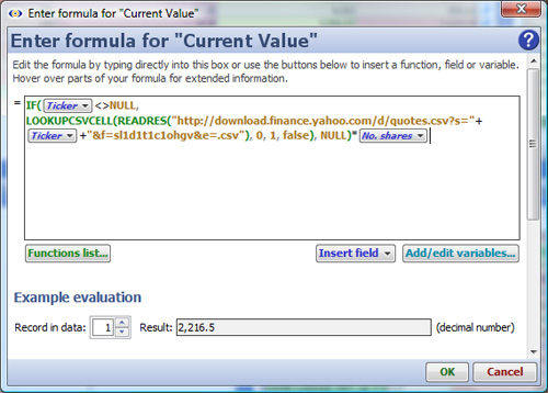
Example: real-time foreign exchange conversions, where [Currency] is the currency pair to be converted in a field in the data set, e.g. GBPUSD. Use the URL below inside a formula syntax similar to the one shown in the Formula Editor screenshot above:
http://download.finance.yahoo.com/d/quotes.csv?s="+[Currency]+"=X&f=sl1d1t1c1ohgv&e=.csv
Note: when preparing your data sets, be aware of the upper/lower case sensitivity for any web services you plan to draw on. Test the format of the input parameter before preparing your data. For example, the sample web services links below all require a lowercase U.S. stock ticker symbol. Add as many web services as you want, using any number of Omniscope Web Views to display the automatically-generated results from posting the user-selected row values as inputs. If necessary, use Omniscope Operations tools like Summarise fields or Expand/Collapse fields to modify your data to match the required format of the web service input parameter.
The services below all accept a lowercase US stock ticker as the web service parameter:
Table Chart: for each Symbol, returns Last Trade, Trade Time, Change, Volume and Todays Price:
http://appsupport.visokio.com/appsupport/symbolPrices.cfm [134]
Line Chart: for each Symbol, shows Price over time for the day:
http://appsupport.visokio.com/appsupport/yahooFinanceTodaysPrice.cfm [135]
Line Chart: for each Symbol, shows Price over the past year:
http://appsupport.visokio.com/appsupport/yahooFinanceYearPrice.cfm [136]
Omniscope includes a test web service that 'echos' whatever field (column) of values are selected in the current tab. Try configuring this web service using the default Visokio URL given, with a name like 'Echo Test', and select any field in your data set. Switch to one of the views in Omniscope, and select less than 100 records, then (on the newly-added Main Toolbar web services menu button) click on the 'Echo Test' web service button. If you have configured a Web View to display the web service results, they will appear in that open Web View. If you have not configured a Web View in Omniscope, your default browser will open and display the echo results, which are being returned from a Visokio server.
This section lists functions available in earlier versions of Omniscope which have been classified as "deprecated". Although these functions still work, there are now better ways of achieving the same result in more recent versions of Omniscope. These will continue to be supported for the medium term but may be withdrawn from Omniscope after several major releases.
See also: Non-deprecated functions [137] Guide to SUBSET (replacing DATASET) functions [106]
Function | Usage | Description |
| DATASET_EMPTYCOUNT | DATASET_EMPTYCOUNT(stat_field, subset_field, subset_field_value) | Calculates the statistical function [Number of empty values] of a field. Either: (a) for all records (if only stat_field is specified); or (b) for a current subset of records (if subset_field is specified); or (c) for another subset of records (if subset_field and subset_field_value are specified). Deprecated - please use the SUBSET family of functions instead. |
| DATASET_EMPTYCOUNT2 | DATASET_EMPTYCOUNT2(stat_field, subset_field_1, subset_field_2, subset_field_1_value, subset_field_2_value) | Calculates the statistical function [Number of empty values] of a field. Either: (a) for a current subset of records (if subset_field_N is specified); or (b) for another subset of records (if subset_field_N and subset_field_N_value are specified). Deprecated - please use the SUBSET family of functions instead. |
| DATASET_EMPTYCOUNT3 | DATASET_EMPTYCOUNT3(stat_field, subset_field_1, subset_field_2, subset_field_3, subset_field_1_value, subset_field_2_value, subset_field_3_value) | Calculates the statistical function [Number of empty values] of a field. Either: (a) for a current subset of records (if subset_field_N is specified); or (b) for another subset of records (if subset_field_N and subset_field_N_value are specified). Deprecated - please use the SUBSET family of functions instead. |
| DATASET_EMPTYCOUNT4 | DATASET_EMPTYCOUNT4(stat_field, subset_field_1, subset_field_2, subset_field_3, subset_field_4, subset_field_1_value, subset_field_2_value, subset_field_3_value, subset_field_4_value) | Calculates the statistical function [Number of empty values] of a field. Either: (a) for a current subset of records (if subset_field_N is specified); or (b) for another subset of records (if subset_field_N and subset_field_N_value are specified). Deprecated - please use the SUBSET family of functions instead. |
| DATASET_EMPTYCOUNT5 | DATASET_EMPTYCOUNT5(stat_field, subset_field_1, subset_field_2, subset_field_3, subset_field_4, subset_field_5, subset_field_1_value, subset_field_2_value, subset_field_3_value, subset_field_4_value, subset_field_5_value) | Calculates the statistical function [Number of empty values] of a field. Either: (a) for a current subset of records (if subset_field_N is specified); or (b) for another subset of records (if subset_field_N and subset_field_N_value are specified). Deprecated - please use the SUBSET family of functions instead. |
| DATASET_MAX | DATASET_MAX(stat_field, subset_field, subset_field_value) | Calculates the statistical function [Maximum value (highest or last)] of a field. Either: (a) for all records (if only stat_field is specified); or (b) for a current subset of records (if subset_field is specified); or (c) for another subset of records (if subset_field and subset_field_value are specified). Deprecated - please use the SUBSET family of functions instead. |
| DATASET_MAX2 | DATASET_MAX2(stat_field, subset_field_1, subset_field_2, subset_field_1_value, subset_field_2_value) | Calculates the statistical function [Maximum value (highest or last)] of a field. Either: (a) for a current subset of records (if subset_field_N is specified); or (b) for another subset of records (if subset_field_N and subset_field_N_value are specified). Deprecated - please use the SUBSET family of functions instead. |
| DATASET_MAX3 | DATASET_MAX3(stat_field, subset_field_1, subset_field_2, subset_field_3, subset_field_1_value, subset_field_2_value, subset_field_3_value) | Calculates the statistical function [Maximum value (highest or last)] of a field. Either: (a) for a current subset of records (if subset_field_N is specified); or (b) for another subset of records (if subset_field_N and subset_field_N_value are specified). Deprecated - please use the SUBSET family of functions instead. |
| DATASET_MAX4 | DATASET_MAX4(stat_field, subset_field_1, subset_field_2, subset_field_3, subset_field_4, subset_field_1_value, subset_field_2_value, subset_field_3_value, subset_field_4_value) | Calculates the statistical function [Maximum value (highest or last)] of a field. Either: (a) for a current subset of records (if subset_field_N is specified); or (b) for another subset of records (if subset_field_N and subset_field_N_value are specified). Deprecated - please use the SUBSET family of functions instead. |
| DATASET_MAX5 | DATASET_MAX5(stat_field, subset_field_1, subset_field_2, subset_field_3, subset_field_4, subset_field_5, subset_field_1_value, subset_field_2_value, subset_field_3_value, subset_field_4_value, subset_field_5_value) | Calculates the statistical function [Maximum value (highest or last)] of a field. Either: (a) for a current subset of records (if subset_field_N is specified); or (b) for another subset of records (if subset_field_N and subset_field_N_value are specified). Deprecated - please use the SUBSET family of functions instead. |
| DATASET_MEAN | DATASET_MEAN(stat_field, subset_field, subset_field_value) | Calculates the statistical function [Mean (average) of values] of a field. Either: (a) for all records (if only stat_field is specified); or (b) for a current subset of records (if subset_field is specified); or (c) for another subset of records (if subset_field and subset_field_value are specified). Deprecated - please use the SUBSET family of functions instead. |
| DATASET_MEAN2 | DATASET_MEAN2(stat_field, subset_field_1, subset_field_2, subset_field_1_value, subset_field_2_value) | Calculates the statistical function [Mean (average) of values] of a field. Either: (a) for a current subset of records (if subset_field_N is specified); or (b) for another subset of records (if subset_field_N and subset_field_N_value are specified). Deprecated - please use the SUBSET family of functions instead. |
| DATASET_MEAN3 | DATASET_MEAN3(stat_field, subset_field_1, subset_field_2, subset_field_3, subset_field_1_value, subset_field_2_value, subset_field_3_value) | Calculates the statistical function [Mean (average) of values] of a field. Either: (a) for a current subset of records (if subset_field_N is specified); or (b) for another subset of records (if subset_field_N and subset_field_N_value are specified). Deprecated - please use the SUBSET family of functions instead. |
| DATASET_MEAN4 | DATASET_MEAN4(stat_field, subset_field_1, subset_field_2, subset_field_3, subset_field_4, subset_field_1_value, subset_field_2_value, subset_field_3_value, subset_field_4_value) | Calculates the statistical function [Mean (average) of values] of a field. Either: (a) for a current subset of records (if subset_field_N is specified); or (b) for another subset of records (if subset_field_N and subset_field_N_value are specified). Deprecated - please use the SUBSET family of functions instead. |
| DATASET_MEAN5 | DATASET_MEAN5(stat_field, subset_field_1, subset_field_2, subset_field_3, subset_field_4, subset_field_5, subset_field_1_value, subset_field_2_value, subset_field_3_value, subset_field_4_value, subset_field_5_value) | Calculates the statistical function [Mean (average) of values] of a field. Either: (a) for a current subset of records (if subset_field_N is specified); or (b) for another subset of records (if subset_field_N and subset_field_N_value are specified). Deprecated - please use the SUBSET family of functions instead. |
| DATASET_MEDIAN | DATASET_MEDIAN(stat_field, subset_field, subset_field_value) | Calculates the statistical function [Median (middle) of values] of a field. Either: (a) for all records (if only stat_field is specified); or (b) for a current subset of records (if subset_field is specified); or (c) for another subset of records (if subset_field and subset_field_value are specified). Deprecated - please use the SUBSET family of functions instead. |
| DATASET_MEDIAN2 | DATASET_MEDIAN2(stat_field, subset_field_1, subset_field_2, subset_field_1_value, subset_field_2_value) | Calculates the statistical function [Median (middle) of values] of a field. Either: (a) for a current subset of records (if subset_field_N is specified); or (b) for another subset of records (if subset_field_N and subset_field_N_value are specified). Deprecated - please use the SUBSET family of functions instead. |
| DATASET_MEDIAN3 | DATASET_MEDIAN3(stat_field, subset_field_1, subset_field_2, subset_field_3, subset_field_1_value, subset_field_2_value, subset_field_3_value) | Calculates the statistical function [Median (middle) of values] of a field. Either: (a) for a current subset of records (if subset_field_N is specified); or (b) for another subset of records (if subset_field_N and subset_field_N_value are specified). Deprecated - please use the SUBSET family of functions instead. |
| DATASET_MEDIAN4 | DATASET_MEDIAN4(stat_field, subset_field_1, subset_field_2, subset_field_3, subset_field_4, subset_field_1_value, subset_field_2_value, subset_field_3_value, subset_field_4_value) | Calculates the statistical function [Median (middle) of values] of a field. Either: (a) for a current subset of records (if subset_field_N is specified); or (b) for another subset of records (if subset_field_N and subset_field_N_value are specified). Deprecated - please use the SUBSET family of functions instead. |
| DATASET_MEDIAN5 | DATASET_MEDIAN5(stat_field, subset_field_1, subset_field_2, subset_field_3, subset_field_4, subset_field_5, subset_field_1_value, subset_field_2_value, subset_field_3_value, subset_field_4_value, subset_field_5_value) | Calculates the statistical function [Median (middle) of values] of a field. Either: (a) for a current subset of records (if subset_field_N is specified); or (b) for another subset of records (if subset_field_N and subset_field_N_value are specified). Deprecated - please use the SUBSET family of functions instead. |
| DATASET_MIN | DATASET_MIN(stat_field, subset_field, subset_field_value) | Calculates the statistical function [Minimum value (lowest or first)] of a field. Either: (a) for all records (if only stat_field is specified); or (b) for a current subset of records (if subset_field is specified); or (c) for another subset of records (if subset_field and subset_field_value are specified). Deprecated - please use the SUBSET family of functions instead. |
| DATASET_MIN2 | DATASET_MIN2(stat_field, subset_field_1, subset_field_2, subset_field_1_value, subset_field_2_value) | Calculates the statistical function [Minimum value (lowest or first)] of a field. Either: (a) for a current subset of records (if subset_field_N is specified); or (b) for another subset of records (if subset_field_N and subset_field_N_value are specified). Deprecated - please use the SUBSET family of functions instead. |
| DATASET_MIN3 | DATASET_MIN3(stat_field, subset_field_1, subset_field_2, subset_field_3, subset_field_1_value, subset_field_2_value, subset_field_3_value) | Calculates the statistical function [Minimum value (lowest or first)] of a field. Either: (a) for a current subset of records (if subset_field_N is specified); or (b) for another subset of records (if subset_field_N and subset_field_N_value are specified). Deprecated - please use the SUBSET family of functions instead. |
| DATASET_MIN4 | DATASET_MIN4(stat_field, subset_field_1, subset_field_2, subset_field_3, subset_field_4, subset_field_1_value, subset_field_2_value, subset_field_3_value, subset_field_4_value) | Calculates the statistical function [Minimum value (lowest or first)] of a field. Either: (a) for a current subset of records (if subset_field_N is specified); or (b) for another subset of records (if subset_field_N and subset_field_N_value are specified). Deprecated - please use the SUBSET family of functions instead. |
| DATASET_MIN5 | DATASET_MIN5(stat_field, subset_field_1, subset_field_2, subset_field_3, subset_field_4, subset_field_5, subset_field_1_value, subset_field_2_value, subset_field_3_value, subset_field_4_value, subset_field_5_value) | Calculates the statistical function [Minimum value (lowest or first)] of a field. Either: (a) for a current subset of records (if subset_field_N is specified); or (b) for another subset of records (if subset_field_N and subset_field_N_value are specified). Deprecated - please use the SUBSET family of functions instead. |
| DATASET_MODE | DATASET_MODE(stat_field, subset_field, subset_field_value) | Calculates the statistical function [Most common value (first if multimodal)] of a field. Either: (a) for all records (if only stat_field is specified); or (b) for a current subset of records (if subset_field is specified); or (c) for another subset of records (if subset_field and subset_field_value are specified). Deprecated - please use the SUBSET family of functions instead. |
| DATASET_MODE2 | DATASET_MODE2(stat_field, subset_field_1, subset_field_2, subset_field_1_value, subset_field_2_value) | Calculates the statistical function [Most common value (first if multimodal)] of a field. Either: (a) for a current subset of records (if subset_field_N is specified); or (b) for another subset of records (if subset_field_N and subset_field_N_value are specified). Deprecated - please use the SUBSET family of functions instead. |
| DATASET_MODE3 | DATASET_MODE3(stat_field, subset_field_1, subset_field_2, subset_field_3, subset_field_1_value, subset_field_2_value, subset_field_3_value) | Calculates the statistical function [Most common value (first if multimodal)] of a field. Either: (a) for a current subset of records (if subset_field_N is specified); or (b) for another subset of records (if subset_field_N and subset_field_N_value are specified). Deprecated - please use the SUBSET family of functions instead. |
| DATASET_MODE4 | DATASET_MODE4(stat_field, subset_field_1, subset_field_2, subset_field_3, subset_field_4, subset_field_1_value, subset_field_2_value, subset_field_3_value, subset_field_4_value) | Calculates the statistical function [Most common value (first if multimodal)] of a field. Either: (a) for a current subset of records (if subset_field_N is specified); or (b) for another subset of records (if subset_field_N and subset_field_N_value are specified). Deprecated - please use the SUBSET family of functions instead. |
| DATASET_MODE5 | DATASET_MODE5(stat_field, subset_field_1, subset_field_2, subset_field_3, subset_field_4, subset_field_5, subset_field_1_value, subset_field_2_value, subset_field_3_value, subset_field_4_value, subset_field_5_value) | Calculates the statistical function [Most common value (first if multimodal)] of a field. Either: (a) for a current subset of records (if subset_field_N is specified); or (b) for another subset of records (if subset_field_N and subset_field_N_value are specified). Deprecated - please use the SUBSET family of functions instead. |
| DATASET_NONEMPTYCOUNT | DATASET_NONEMPTYCOUNT(stat_field, subset_field, subset_field_value) | Calculates the statistical function [Number of non-empty values] of a field. Either: (a) for all records (if only stat_field is specified); or (b) for a current subset of records (if subset_field is specified); or (c) for another subset of records (if subset_field and subset_field_value are specified). Deprecated - please use the SUBSET family of functions instead. |
| DATASET_NONEMPTYCOUNT2 | DATASET_NONEMPTYCOUNT2(stat_field, subset_field_1, subset_field_2, subset_field_1_value, subset_field_2_value) | Calculates the statistical function [Number of non-empty values] of a field. Either: (a) for a current subset of records (if subset_field_N is specified); or (b) for another subset of records (if subset_field_N and subset_field_N_value are specified). Deprecated - please use the SUBSET family of functions instead. |
| DATASET_NONEMPTYCOUNT3 | DATASET_NONEMPTYCOUNT3(stat_field, subset_field_1, subset_field_2, subset_field_3, subset_field_1_value, subset_field_2_value, subset_field_3_value) | Calculates the statistical function [Number of non-empty values] of a field. Either: (a) for a current subset of records (if subset_field_N is specified); or (b) for another subset of records (if subset_field_N and subset_field_N_value are specified). Deprecated - please use the SUBSET family of functions instead. |
| DATASET_NONEMPTYCOUNT4 | DATASET_NONEMPTYCOUNT4(stat_field, subset_field_1, subset_field_2, subset_field_3, subset_field_4, subset_field_1_value, subset_field_2_value, subset_field_3_value, subset_field_4_value) | Calculates the statistical function [Number of non-empty values] of a field. Either: (a) for a current subset of records (if subset_field_N is specified); or (b) for another subset of records (if subset_field_N and subset_field_N_value are specified). Deprecated - please use the SUBSET family of functions instead. |
| DATASET_NONEMPTYCOUNT5 | DATASET_NONEMPTYCOUNT5(stat_field, subset_field_1, subset_field_2, subset_field_3, subset_field_4, subset_field_5, subset_field_1_value, subset_field_2_value, subset_field_3_value, subset_field_4_value, subset_field_5_value) | Calculates the statistical function [Number of non-empty values] of a field. Either: (a) for a current subset of records (if subset_field_N is specified); or (b) for another subset of records (if subset_field_N and subset_field_N_value are specified). Deprecated - please use the SUBSET family of functions instead. |
| DATASET_PRODUCT | DATASET_PRODUCT(stat_field, subset_field, subset_field_value) | Calculates the statistical function [Product of values] of a field. Either: (a) for all records (if only stat_field is specified); or (b) for a current subset of records (if subset_field is specified); or (c) for another subset of records (if subset_field and subset_field_value are specified). Deprecated - please use the SUBSET family of functions instead. |
| DATASET_PRODUCT2 | DATASET_PRODUCT2(stat_field, subset_field_1, subset_field_2, subset_field_1_value, subset_field_2_value) | Calculates the statistical function [Product of values] of a field. Either: (a) for a current subset of records (if subset_field_N is specified); or (b) for another subset of records (if subset_field_N and subset_field_N_value are specified). Deprecated - please use the SUBSET family of functions instead. |
| DATASET_PRODUCT3 | DATASET_PRODUCT3(stat_field, subset_field_1, subset_field_2, subset_field_3, subset_field_1_value, subset_field_2_value, subset_field_3_value) | Calculates the statistical function [Product of values] of a field. Either: (a) for a current subset of records (if subset_field_N is specified); or (b) for another subset of records (if subset_field_N and subset_field_N_value are specified). Deprecated - please use the SUBSET family of functions instead. |
| DATASET_PRODUCT4 | DATASET_PRODUCT4(stat_field, subset_field_1, subset_field_2, subset_field_3, subset_field_4, subset_field_1_value, subset_field_2_value, subset_field_3_value, subset_field_4_value) | Calculates the statistical function [Product of values] of a field. Either: (a) for a current subset of records (if subset_field_N is specified); or (b) for another subset of records (if subset_field_N and subset_field_N_value are specified). Deprecated - please use the SUBSET family of functions instead. |
| DATASET_PRODUCT5 | DATASET_PRODUCT5(stat_field, subset_field_1, subset_field_2, subset_field_3, subset_field_4, subset_field_5, subset_field_1_value, subset_field_2_value, subset_field_3_value, subset_field_4_value, subset_field_5_value) | Calculates the statistical function [Product of values] of a field. Either: (a) for a current subset of records (if subset_field_N is specified); or (b) for another subset of records (if subset_field_N and subset_field_N_value are specified). Deprecated - please use the SUBSET family of functions instead. |
| DATASET_RANGE | DATASET_RANGE(stat_field, subset_field, subset_field_value) | Calculates the statistical function [Range of values (maximum minus minimum)] of a field. Either: (a) for all records (if only stat_field is specified); or (b) for a current subset of records (if subset_field is specified); or (c) for another subset of records (if subset_field and subset_field_value are specified). Deprecated - please use the SUBSET family of functions instead. |
| DATASET_RANGE2 | DATASET_RANGE2(stat_field, subset_field_1, subset_field_2, subset_field_1_value, subset_field_2_value) | Calculates the statistical function [Range of values (maximum minus minimum)] of a field. Either: (a) for a current subset of records (if subset_field_N is specified); or (b) for another subset of records (if subset_field_N and subset_field_N_value are specified). Deprecated - please use the SUBSET family of functions instead. |
| DATASET_RANGE3 | DATASET_RANGE3(stat_field, subset_field_1, subset_field_2, subset_field_3, subset_field_1_value, subset_field_2_value, subset_field_3_value) | Calculates the statistical function [Range of values (maximum minus minimum)] of a field. Either: (a) for a current subset of records (if subset_field_N is specified); or (b) for another subset of records (if subset_field_N and subset_field_N_value are specified). Deprecated - please use the SUBSET family of functions instead. |
| DATASET_RANGE4 | DATASET_RANGE4(stat_field, subset_field_1, subset_field_2, subset_field_3, subset_field_4, subset_field_1_value, subset_field_2_value, subset_field_3_value, subset_field_4_value) | Calculates the statistical function [Range of values (maximum minus minimum)] of a field. Either: (a) for a current subset of records (if subset_field_N is specified); or (b) for another subset of records (if subset_field_N and subset_field_N_value are specified). Deprecated - please use the SUBSET family of functions instead. |
| DATASET_RANGE5 | DATASET_RANGE5(stat_field, subset_field_1, subset_field_2, subset_field_3, subset_field_4, subset_field_5, subset_field_1_value, subset_field_2_value, subset_field_3_value, subset_field_4_value, subset_field_5_value) | Calculates the statistical function [Range of values (maximum minus minimum)] of a field. Either: (a) for a current subset of records (if subset_field_N is specified); or (b) for another subset of records (if subset_field_N and subset_field_N_value are specified). Deprecated - please use the SUBSET family of functions instead. |
| DATASET_RECORDCOUNT | DATASET_RECORDCOUNT(stat_field, subset_field, subset_field_value) | Calculates the statistical function [Number of records] of a field. Either: (a) for all records (if only stat_field is specified); or (b) for a current subset of records (if subset_field is specified); or (c) for another subset of records (if subset_field and subset_field_value are specified). Deprecated - please use the SUBSET family of functions instead. |
| DATASET_RECORDCOUNT2 | DATASET_RECORDCOUNT2(stat_field, subset_field_1, subset_field_2, subset_field_1_value, subset_field_2_value) | Calculates the statistical function [Number of records] of a field. Either: (a) for a current subset of records (if subset_field_N is specified); or (b) for another subset of records (if subset_field_N and subset_field_N_value are specified). Deprecated - please use the SUBSET family of functions instead. |
| DATASET_RECORDCOUNT3 | DATASET_RECORDCOUNT3(stat_field, subset_field_1, subset_field_2, subset_field_3, subset_field_1_value, subset_field_2_value, subset_field_3_value) | Calculates the statistical function [Number of records] of a field. Either: (a) for a current subset of records (if subset_field_N is specified); or (b) for another subset of records (if subset_field_N and subset_field_N_value are specified). Deprecated - please use the SUBSET family of functions instead. |
| DATASET_RECORDCOUNT4 | DATASET_RECORDCOUNT4(stat_field, subset_field_1, subset_field_2, subset_field_3, subset_field_4, subset_field_1_value, subset_field_2_value, subset_field_3_value, subset_field_4_value) | Calculates the statistical function [Number of records] of a field. Either: (a) for a current subset of records (if subset_field_N is specified); or (b) for another subset of records (if subset_field_N and subset_field_N_value are specified). Deprecated - please use the SUBSET family of functions instead. |
| DATASET_RECORDCOUNT5 | DATASET_RECORDCOUNT5(stat_field, subset_field_1, subset_field_2, subset_field_3, subset_field_4, subset_field_5, subset_field_1_value, subset_field_2_value, subset_field_3_value, subset_field_4_value, subset_field_5_value) | Calculates the statistical function [Number of records] of a field. Either: (a) for a current subset of records (if subset_field_N is specified); or (b) for another subset of records (if subset_field_N and subset_field_N_value are specified). Deprecated - please use the SUBSET family of functions instead. |
| DATASET_SINGLETON | DATASET_SINGLETON(stat_field, subset_field, subset_field_value) | Calculates the statistical function [The single value, if there is one] of a field. Either: (a) for all records (if only stat_field is specified); or (b) for a current subset of records (if subset_field is specified); or (c) for another subset of records (if subset_field and subset_field_value are specified). Deprecated - please use the SUBSET family of functions instead. |
| DATASET_SINGLETON2 | DATASET_SINGLETON2(stat_field, subset_field_1, subset_field_2, subset_field_1_value, subset_field_2_value) | Calculates the statistical function [The single value, if there is one] of a field. Either: (a) for a current subset of records (if subset_field_N is specified); or (b) for another subset of records (if subset_field_N and subset_field_N_value are specified). Deprecated - please use the SUBSET family of functions instead. |
| DATASET_SINGLETON3 | DATASET_SINGLETON3(stat_field, subset_field_1, subset_field_2, subset_field_3, subset_field_1_value, subset_field_2_value, subset_field_3_value) | Calculates the statistical function [The single value, if there is one] of a field. Either: (a) for a current subset of records (if subset_field_N is specified); or (b) for another subset of records (if subset_field_N and subset_field_N_value are specified). Deprecated - please use the SUBSET family of functions instead. |
| DATASET_SINGLETON4 | DATASET_SINGLETON4(stat_field, subset_field_1, subset_field_2, subset_field_3, subset_field_4, subset_field_1_value, subset_field_2_value, subset_field_3_value, subset_field_4_value) | Calculates the statistical function [The single value, if there is one] of a field. Either: (a) for a current subset of records (if subset_field_N is specified); or (b) for another subset of records (if subset_field_N and subset_field_N_value are specified). Deprecated - please use the SUBSET family of functions instead. |
| DATASET_SINGLETON5 | DATASET_SINGLETON5(stat_field, subset_field_1, subset_field_2, subset_field_3, subset_field_4, subset_field_5, subset_field_1_value, subset_field_2_value, subset_field_3_value, subset_field_4_value, subset_field_5_value) | Calculates the statistical function [The single value, if there is one] of a field. Either: (a) for a current subset of records (if subset_field_N is specified); or (b) for another subset of records (if subset_field_N and subset_field_N_value are specified). Deprecated - please use the SUBSET family of functions instead. |
| DATASET_STDDEV | DATASET_STDDEV(stat_field, subset_field, subset_field_value) | Calculates the statistical function [Standard deviation of values from the mean] of a field. Either: (a) for all records (if only stat_field is specified); or (b) for a current subset of records (if subset_field is specified); or (c) for another subset of records (if subset_field and subset_field_value are specified). Deprecated - please use the SUBSET family of functions instead. |
| DATASET_STDDEV2 | DATASET_STDDEV2(stat_field, subset_field_1, subset_field_2, subset_field_1_value, subset_field_2_value) | Calculates the statistical function [Standard deviation of values from the mean] of a field. Either: (a) for a current subset of records (if subset_field_N is specified); or (b) for another subset of records (if subset_field_N and subset_field_N_value are specified). Deprecated - please use the SUBSET family of functions instead. |
| DATASET_STDDEV3 | DATASET_STDDEV3(stat_field, subset_field_1, subset_field_2, subset_field_3, subset_field_1_value, subset_field_2_value, subset_field_3_value) | Calculates the statistical function [Standard deviation of values from the mean] of a field. Either: (a) for a current subset of records (if subset_field_N is specified); or (b) for another subset of records (if subset_field_N and subset_field_N_value are specified). Deprecated - please use the SUBSET family of functions instead. |
| DATASET_STDDEV4 | DATASET_STDDEV4(stat_field, subset_field_1, subset_field_2, subset_field_3, subset_field_4, subset_field_1_value, subset_field_2_value, subset_field_3_value, subset_field_4_value) | Calculates the statistical function [Standard deviation of values from the mean] of a field. Either: (a) for a current subset of records (if subset_field_N is specified); or (b) for another subset of records (if subset_field_N and subset_field_N_value are specified). Deprecated - please use the SUBSET family of functions instead. |
| DATASET_STDDEV5 | DATASET_STDDEV5(stat_field, subset_field_1, subset_field_2, subset_field_3, subset_field_4, subset_field_5, subset_field_1_value, subset_field_2_value, subset_field_3_value, subset_field_4_value, subset_field_5_value) | Calculates the statistical function [Standard deviation of values from the mean] of a field. Either: (a) for a current subset of records (if subset_field_N is specified); or (b) for another subset of records (if subset_field_N and subset_field_N_value are specified). Deprecated - please use the SUBSET family of functions instead. |
| DATASET_SUM | DATASET_SUM(stat_field, subset_field, subset_field_value) | Calculates the statistical function [Sum (total) of values] of a field. Either: (a) for all records (if only stat_field is specified); or (b) for a current subset of records (if subset_field is specified); or (c) for another subset of records (if subset_field and subset_field_value are specified). Deprecated - please use the SUBSET family of functions instead. |
| DATASET_SUM2 | DATASET_SUM2(stat_field, subset_field_1, subset_field_2, subset_field_1_value, subset_field_2_value) | Calculates the statistical function [Sum (total) of values] of a field. Either: (a) for a current subset of records (if subset_field_N is specified); or (b) for another subset of records (if subset_field_N and subset_field_N_value are specified). Deprecated - please use the SUBSET family of functions instead. |
| DATASET_SUM3 | DATASET_SUM3(stat_field, subset_field_1, subset_field_2, subset_field_3, subset_field_1_value, subset_field_2_value, subset_field_3_value) | Calculates the statistical function [Sum (total) of values] of a field. Either: (a) for a current subset of records (if subset_field_N is specified); or (b) for another subset of records (if subset_field_N and subset_field_N_value are specified). Deprecated - please use the SUBSET family of functions instead. |
| DATASET_SUM4 | DATASET_SUM4(stat_field, subset_field_1, subset_field_2, subset_field_3, subset_field_4, subset_field_1_value, subset_field_2_value, subset_field_3_value, subset_field_4_value) | Calculates the statistical function [Sum (total) of values] of a field. Either: (a) for a current subset of records (if subset_field_N is specified); or (b) for another subset of records (if subset_field_N and subset_field_N_value are specified). Deprecated - please use the SUBSET family of functions instead. |
| DATASET_SUM5 | DATASET_SUM5(stat_field, subset_field_1, subset_field_2, subset_field_3, subset_field_4, subset_field_5, subset_field_1_value, subset_field_2_value, subset_field_3_value, subset_field_4_value, subset_field_5_value) | Calculates the statistical function [Sum (total) of values] of a field. Either: (a) for a current subset of records (if subset_field_N is specified); or (b) for another subset of records (if subset_field_N and subset_field_N_value are specified). Deprecated - please use the SUBSET family of functions instead. |
| DATASET_UNIQUECOUNT | DATASET_UNIQUECOUNT(stat_field, subset_field, subset_field_value) | Calculates the statistical function [Number of unique non-empty values] of a field. Either: (a) for all records (if only stat_field is specified); or (b) for a current subset of records (if subset_field is specified); or (c) for another subset of records (if subset_field and subset_field_value are specified). Deprecated - please use the SUBSET family of functions instead. |
| DATASET_UNIQUECOUNT2 | DATASET_UNIQUECOUNT2(stat_field, subset_field_1, subset_field_2, subset_field_1_value, subset_field_2_value) | Calculates the statistical function [Number of unique non-empty values] of a field. Either: (a) for a current subset of records (if subset_field_N is specified); or (b) for another subset of records (if subset_field_N and subset_field_N_value are specified). Deprecated - please use the SUBSET family of functions instead. |
| DATASET_UNIQUECOUNT3 | DATASET_UNIQUECOUNT3(stat_field, subset_field_1, subset_field_2, subset_field_3, subset_field_1_value, subset_field_2_value, subset_field_3_value) | Calculates the statistical function [Number of unique non-empty values] of a field. Either: (a) for a current subset of records (if subset_field_N is specified); or (b) for another subset of records (if subset_field_N and subset_field_N_value are specified). Deprecated - please use the SUBSET family of functions instead. |
| DATASET_UNIQUECOUNT4 | DATASET_UNIQUECOUNT4(stat_field, subset_field_1, subset_field_2, subset_field_3, subset_field_4, subset_field_1_value, subset_field_2_value, subset_field_3_value, subset_field_4_value) | Calculates the statistical function [Number of unique non-empty values] of a field. Either: (a) for a current subset of records (if subset_field_N is specified); or (b) for another subset of records (if subset_field_N and subset_field_N_value are specified). Deprecated - please use the SUBSET family of functions instead. |
| DATASET_UNIQUECOUNT5 | DATASET_UNIQUECOUNT5(stat_field, subset_field_1, subset_field_2, subset_field_3, subset_field_4, subset_field_5, subset_field_1_value, subset_field_2_value, subset_field_3_value, subset_field_4_value, subset_field_5_value) | Calculates the statistical function [Number of unique non-empty values] of a field. Either: (a) for a current subset of records (if subset_field_N is specified); or (b) for another subset of records (if subset_field_N and subset_field_N_value are specified). Deprecated - please use the SUBSET family of functions instead. |
| DATASET_UNIQUESLIST | DATASET_UNIQUESLIST(stat_field, subset_field, subset_field_value) | Calculates the statistical function [A comma-separated list of all unique values] of a field. Either: (a) for all records (if only stat_field is specified); or (b) for a current subset of records (if subset_field is specified); or (c) for another subset of records (if subset_field and subset_field_value are specified). Deprecated - please use the SUBSET family of functions instead. |
| DATASET_UNIQUESLIST2 | DATASET_UNIQUESLIST2(stat_field, subset_field_1, subset_field_2, subset_field_1_value, subset_field_2_value) | Calculates the statistical function [A comma-separated list of all unique values] of a field. Either: (a) for a current subset of records (if subset_field_N is specified); or (b) for another subset of records (if subset_field_N and subset_field_N_value are specified). Deprecated - please use the SUBSET family of functions instead. |
| DATASET_UNIQUESLIST3 | DATASET_UNIQUESLIST3(stat_field, subset_field_1, subset_field_2, subset_field_3, subset_field_1_value, subset_field_2_value, subset_field_3_value) | Calculates the statistical function [A comma-separated list of all unique values] of a field. Either: (a) for a current subset of records (if subset_field_N is specified); or (b) for another subset of records (if subset_field_N and subset_field_N_value are specified). Deprecated - please use the SUBSET family of functions instead. |
| DATASET_UNIQUESLIST4 | DATASET_UNIQUESLIST4(stat_field, subset_field_1, subset_field_2, subset_field_3, subset_field_4, subset_field_1_value, subset_field_2_value, subset_field_3_value, subset_field_4_value) | Calculates the statistical function [A comma-separated list of all unique values] of a field. Either: (a) for a current subset of records (if subset_field_N is specified); or (b) for another subset of records (if subset_field_N and subset_field_N_value are specified). Deprecated - please use the SUBSET family of functions instead. |
| DATASET_UNIQUESLIST5 | DATASET_UNIQUESLIST5(stat_field, subset_field_1, subset_field_2, subset_field_3, subset_field_4, subset_field_5, subset_field_1_value, subset_field_2_value, subset_field_3_value, subset_field_4_value, subset_field_5_value) | Calculates the statistical function [A comma-separated list of all unique values] of a field. Either: (a) for a current subset of records (if subset_field_N is specified); or (b) for another subset of records (if subset_field_N and subset_field_N_value are specified). Deprecated - please use the SUBSET family of functions instead. |
| SUBSET_RECORDCOUNT (Omniscope 2.5+) |
SUBSET_RECORDCOUNT(stat_field, subset) In scripts: subset_recordCount(stat_field, subset) |
Calculates the statistical function [Number of records] of a field. Either: (a) for all records (if only field_name is specified); or (b) for a subset of data (if subset is specified). Use the SUBSET function to define a data subset. Deprecated - please use the RECORDCOUNT function instead. For more information, please visit SUBSET functions [106]. |
The DATASET_... functions (documented in Deprecated Functions [107]) were deprecated as of verson 2.5. New SUBSET functions, in combination with other existing functions, are more flexible and efficient.
See also: Functions Guide [137] Guide to SUBSET functions [106] Deprecated Functions [107]
The Formula Editor dialog in Omniscope is a powerful tool for creating and editing an Omniscope formula. For more general information about adding formulae to your files, see Formula Fields [30].
The large white box is the formula itself. This box can be edited just like a text field in a form. You can type your formula in from scratch, or use the buttons underneath to help you insert elements of the formula.
Field and variable references are shown inside the text as little embedded buttons, but these behave like characters in the text, and can be selected, cut, copied, pasted and deleted just like other text. Additionally, you can click each embedded button to change the field or variable.
Field references can be inserted using the Insert field below the formula box. Variable [104] references can be inserted using Insert variable except you will need to define the variable beforehand using Add/edit variables [104].
Alternatively, you can type the field/variable name directly (but if it has punctuation or spaces, you will need to enclose the name in [square brackets]).
Colours are used to identify different parts of the formula. For example, green indicates a function such as SUM(...), blue indicates a field reference, and cyan/turquoise indicates a variable reference.
During a session with the formula editor, use Ctrl+Z to undo your edits, and Ctrl+Y or Ctrl+Shift+Z to redo edits you have undone. Accidentally deleted half an hour's work? Ctrl+Z will bring it back.
Once you have clicked OK, the edited formula will be applied and your fields will recalculate. At this point, from the main Omniscope window, you can use Data > Undo edit or press Ctrl+Z to undo the entire formula editing session (from the point you opened the formula editor until you pressed OK).
If you know the function, simply type its name followed by an open bracket, e.g. "SUM(". Then provide any arguments/parameters to the function, separated by commas, ending with a close bracket. For example: "SUM(1, 2)".
If you are unsure how to use a particular function, type the function name and the open bracket, then move your mouse over the function. A tooltip will appear with guidance.
To browse and insert functions from a list, click Functions list [138]. In the dialog that appears, browse through the functions and read their syntax. Find the function you want and click OK. The function and sample usage will be inserted into the formula at the cursor position. This will typically introduce errors which will be highlighted, since you must change the sample argument/parameter names for real values, references or expressions. More... [138]
All standard spreadsheet functions are provided where appropriate for Omniscope, so you can expect POWER() to work in the same way as Excel, for example. Additional Omniscope-specific functions such as SUBSET are also provided.
See the Knowledge Base Functions Guide [102] for full documentation of all functions.
Long and complicated formulae can be hard to read and work with. Use spaces, tabs, line-breaks and comments to space-out and describe sections of the formula, without affecting calculation.
Comments must be surrounded with "/*" and "*/" as in the following example:
(1 + 1) /* adding some numbers */
/ 2 /* dividing in half */
The formula editor window can also be resized as large as needed when working on a very large formula.
While editing your formula, you can see the results in two ways:
In the section Example evaluation, use the Record in data spinner to select a record. Providing your formula has no errors, the result will be shown to the right, along with the data type. If you move the formula editor to one side, the same record will be highlighted in the views.
Move your mouse over the formula. As you move, different parts will become highlighted, and if you hold the mouse over a particular part, a tooltip will appear containing the result of that part of the formula when evaluated against the record chosen in Example evaluation.
For example, in the formula "(1 + 1) * 2", moving your mouse over the "+" will highlight "1 + 1" and the tooltip will show "1 + 1 = 2". Moving over the "*" will highlight "(1 + 1) * 2", and the tooltip will show "(1 + 1) * 2 = 4".
If your formula contains errors, these will be reported in red text in the Errors section. Guidance text deemed useful for a function in the formula will be shown. The relevant part of the formula will be highlighted in pink.
Omniscope contains an extensive list of standard and specialised functions you can use to define Formula fields. In addition to the standard functions (with the same syntax) found in spreadsheets like Excel, Omniscope also contains a library of powerful DATASET functions that operate on one or more columns and can define the subset of data for which calculations should be be done based on values in other columns.
In the Formula Editor [103], choose Functions list to see the following dialog.
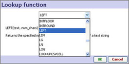 | 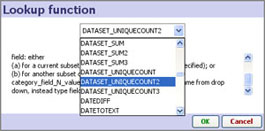 |
Each function is documented briefly in the functions list. For online documentation of available functions, including more detailed documentation of Omniscope-specific functions such as SUBSET(), consult our Functions Guide [29].
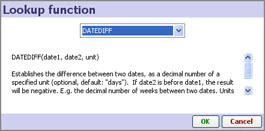 | 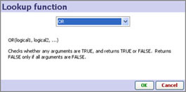 |
If you have questions about how to define formulae for specific tasks, consult the KnowledgeBase Useful Formulae [105] section. If you would like to propose additional functions you would find helpful, please post your ideas in the Forums [139] page.
Omniscope permits extremely powerful modelling with multiple sensitivity analyses in real-time using Variables you can define and insert in formula fields [30].
AS defined in Omniscope, Variables are input assumptions (not fields in the data set) you define by setting a default value and specifying upper and lower ranges. Variables are used as flexible assumption values (as opposed to factual/historic values in the data set) for making dynamic sensitivity analyses and real-time modelling options available to users of the file.
The value used in formulae containing variables can be modified by your users from the initial default using the Side Bar sliders corresponding to each variable. These sliders must be visible (ticked in the Devices drop-down menu on the Side Bar) in order for you and your users to 'flex' the assumptions by adjusting the current value of the variable. Any variable whose current value is different from the default will show a highlighted Side Bar slider device, as with active filter devices. As with filters, clicking Reset on the main toolbar reverts all variables to their configured default values.
Let's look at another example of a formula that uses a different type of Variable. In the example below (taken from the embedded demo presentation 'Cajun Sugar report', where each record is a sugar refinery), the IF function is used to test the 'Energy source' column value. Only if the value equals "Fuel", is the assumption Variable 'Oil Price' used to adjust the energy costs.
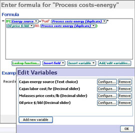 | 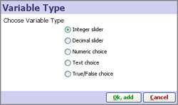 |
You must define Variables before they can be used in expressions defining the values in Formula fields [30]. Click on Add/Edit variables and you will be asked to specify one of 5 types of Variable, each of which has a Side Bar device and other rules associated with it:
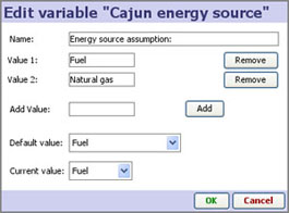 | 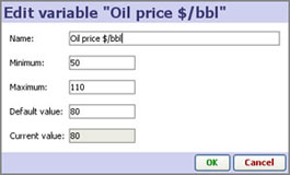 |
Depending on the type of Variable you are specifying, you will be asked to define one or more allowable values, or a range of values with a minimum, maximum and default. If you display the Side Bar devices associated with key input/assumption Variables, users can easily change any or all assumptions and see the calculated quantities and graphic visualisations updated in real time.
To specify different values for Variables, you can use the sliders, or you can type one or more combinations of values directly into the Side Bar. In the example above, notice that the 'Energy source' assumption for one refinery can be changed, and other cost assumptions changed simultaneously. The lack of orange shading on the Side Bar device tells us that the 'Energy source' = "Fuel" assumption is the default. However, the oil price assumption slider is not set to the default value and is therefore shaded orange. If you save this non-default scenario as a Report Page, that Report Page will always open with this mix of default and non-default values- unless you untick the Variable states option under This page will capture: in the Create Page dialog. If you do untick this option, the Report Page will always open with the default values set for all Variables. The user can of course change them at any time.
Note: notice above that all the calculated Formula columns display blue headers in the Table View.
Omniscope allows you to write your own JavaScript to extend Omniscope's functionality in several ways. The current scripting language is JavaScript, and in the case of the DataManager Custom Script block, and the DataExplorer Content View this is 'pure' Javascript without any of the browser-specific objects and methods typically seen in a web page. Scripting inside the Omniscope Web View using browser-friendly JavaScript is discussed here [140].
Using the SCRIPT [141] formula function, you can execute Javascript and invoke formula functions directly from your JavaScript. The last value in your Javascript is used as the return value of the SCRIPT function.
For example:
DEPENDENCIES(

  SCRIPT(`
    // Running total of Coupon field for all Categories up to the current Category:
    var array = subset_uniquesList("Category");
    var total = 0;
    var curval = refVal("Category");
    for (var i in array) {
      var val = array[i];
      total += subset_sum("Coupon", subset("Category", val));
      if (val==curval) break; // Stop here
    }
    // Result value:
    total;
  `),

  /* list of fields referenced by script: */
  [Category], [Coupon]

)
For a full list of supported functions, look for those with "In script" shown in the Functions Guide [102]. Also see here [108] for further JavaScript-specific functions. Note also the use of back-quotes in formulae [142], making it easier to use regular quotes inside the script.
This SCRIPT formula function can be used in the Content View, as measures in the new Bar/Line view, and also in formula fields. If used in formula fields, it is essential to identify any referenced fields inside your script by wrapping the SCRIPT inside a DEPENDENCIES [143] function as shown above. Without this, Omniscope cannot determine the correct calculation sequence.
By editing the page source and using <# #> fragments, you can insert preprocessing commands into your HTML source code. You might use this to create data-driven repeated sections, conditional sections, or entirely new content by writing arbitrary text to the output.
For example:
<##>
You can also write directly to the output. For example:
<#
out.println("<br>"); // add linebreak
out.println("Records: "+recordCount());
#>
This is much like JSP or ASP, with the HTML document effectively preprocessed by the script "server-side" (the "server" being the Content View's data engine, not actually a separate server).
You can also use this within any rich text field supporting formulae, after switching to source mode (edit, and press the "<>" toolbar button):
"Scripting in formulae [144]" Forums discussion
"Scripting in Content View [145]" Forums discussion
"Scripting with arrays of data [146]" Forums discussion
Note: This type of scripting should not be confused with browser scripting within an embedded web browser.
Many standard formula functions are also available for direct use in JavaScript. These are documented in the Functions Guide [102]. Look for "In scripts" in the Usage column.
All functions behave identically to regular formula functions, as documented, with the exception of subset_uniquesList() which returns a Javascript array rather than a comma-separated String. Functions that are not supported can be accessed using formula() - see below - or by requesting it to be upgraded by posting on the forums.
The following functions are not in the functions guide, since they are only available in JavaScript:
formula("IF(RAND<0.5, true, false)")
Dynamically evaluates an arbitrary formula using normal formula syntax. This supports all functions in the functions guide, but you must build up a valid formula as a Javascript String.
dataArray() or dataArray(fields)
or dataArray(fields, rowSubset) or dataArray(fields, rowSubset, includeFieldNames)
For example: dataArray( ["Field 1", "Field 2"], subset("Region", "Europe"), true )
Returns a two-dimensional array of cell data, structured as [column][row], indexed from 0 to n-1. See example [146]. If includeFieldNames is true, the first 'row' will be the field names (the first entry in each column array).
The Omniscope Web Views are browsers that allow browser-friendly scripts in the page content, executed in the system default native browser and embedded within Omniscope, to access certain Omniscope variables, through a global JavaScript object named 'omniscope'. Currently, the current file URL can be retrieved through this mechanism.
This object is only made available after the page has loaded. You should not access it on page load or earlier, and should use a timeout to ensure the value has been set.
The global object is currently as follows:
omniscope = {"currentFileURL" : "http://....."}
omniscope.currentFileURL : represents the current Omniscope IOK file URL
Omniscope is a powerful tool for GIS and locational analytics. From version 2.9, Omniscope includes not only boundary overlay (shapefile) management, but also links to a number of free and subscription cloud-based GIS services, like geo-location and advanced spatial processing on remote servers.
In this section you will find documentation and other resources to help you make the most of the geographic and other coordinate mapping capabilities of Omniscope.
Offline mapping [48] -
Freely-installable vector maps that zoom while the user is offline are available from the Maps Library [48]
Coordinate merge/lookup files [60] -
Lookup or merge files are Omniscope files containing columns of useful data you can quickly add to your own files using merge operations. Geographic coordinates for countries, cities and post codes can be imported into Omniscope files using lookup/merge files like those below.
From version 2.6, the Lookup data menu available from the DataManager workspace contans an increasing number of useful data sets ready to merge into your files. For users of Professional 2.5 and prior, below we offer a free library of Omniscope IOK format merge files containing decimal latitudes and longitude coordinates as well as other useful reference data.
Using images as map backgrounds -
Any image, including street-level screenshots from online mapping services can be imported as an image and used as a map background in Omniscope. Use a reference source like Google Earth to pinpoint the decimal longitude and latitude of the points in the lower left and upper right hand corners of the image, then use Omniscope's Map View: View Tools > Change map projection command to re-calibrate the image to decimal longitude and latitude for correct display of your records on the image. See Projection transformation [147].
Below you will find links to free vector maps for use in Omniscope files. These maps will open and zoom offline as well as online. If you use these maps in a file you send to others, the map will automatically be downloaded and installed on their computer as well.
Almost all these maps now support decimal latitude/longitude coordinates like those used in the Google Maps/Earth mapping options. Maps with names shown in red do not yet support decimal latitude/longitude. Contact us [86] if you need a converted version, or alternatively you can place your record markers manually on these maps.
Note: These city maps do not at present use a common coordinate system and cannot be used with latitude/longitude data. Instead markers must be placed on the map manually using Place markers in the Map view.
| London, centre [358] (467kb) | Paris, lightweight [359] (1.93mb) |
Omniscope comes with a detailed multi-layered world map using a Mercator projection, as shown in the images below. A variation of this map is also available with slightly higher detail and including North American states. Both world maps use the decimal Latitude/Longitude coordinate system.
| World, high detail [361] (6.6mb) | For Robinson and other projections please contact us [360] | |
All Visokio applications include a multi-layer Mercator World Map that supports the decimal latitude and longitude coordinate system. These vector maps can be installed and/or embedded in files to work offline and allow users to zoom in without loss in image quality. Multiple layers allow users of the file to selectively show or hide map detail features such as roads, towns and physical relief...with just a mouse click.
In addition to the included World Map, our Maps Library also includes free country maps for every country in the world, as well as a growing number of city maps. Unless otherwise indicated, these downloadable maps support the Mercator decimal latitude and longitude coordinate system. Some maps in the Library (those not marked with an asterisk) do not yet support this standard. Maps that do not yet support this standard require coordinates to be placed manually using the application. If you need a particular map that is not yet converted to the Mercator decimal projection, please contact us about converting it.
Data sets containing decimal latitude and longitude coordinate columns are plotted on corresponding decimal coordinate maps automatically. Depending on your data set, you may be able to use Merge Files [60] to add geographic coordinate data to your files. Reference sources such as Google Earth and Wikipedia can be used to search for, copy & paste missing coordinates in the appropriate decimal format. Alternatively, missing coordinates can be filled in by placing records on either Visokio embedded or online Google Maps manually, allowing the application to estimate the coordinates and add the data to your file.
In addition to embedded vector maps that work offline, all Visokio applications support creating combined displays or overlays ('mash-ups') using Google Maps while connected to the Internet. Omniscope files can also be used together with Google Earth (experimental feature).
Adding more maps to your locally-installed Visokio maps folder is simple:
If you create and distribute Omniscope project files using Visokio maps, the maps can be embedded, and anyone receiving your files will be prompted to automatically download the required maps from this Maps Library. More information on using maps with Omniscope is available in the User Guide section Using Maps [362].
Lookup or merge files are Omniscope files containing columns of useful data you can quickly add to your own files using merge operations. Geographic coordinates for countries, cities and post codes can be imported into Omniscope files using lookup/merge files like those below.
From version 2.6, the Lookup data menu available from the DataManager workspace contans an increasing number of useful data sets ready to merge into your files. For users of Professional 2.5 and prior, below we offer a free library of Omniscope IOK format merge files containing decimal latitudes and longitude coordinates as well as other useful reference data.
Add data columns such as the latitudes and longitudes of capital or major cities or the geographic centres of countries to your files automatically using our By Countries, By Cities or By Post Codes merge files. Once merged into your data sets, these addtional columns of geographic coordinates permit your records to be plotted automaticaly in the Map View, using either embedded vector maps (that work offline) or the zooming online mapping services available in the Map View.
Map Coordinates by ISO Country Codes (with capital cities):
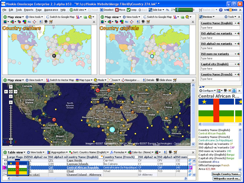 [363] [363](click for larger image) |
Use this free merge file to import decimal map coordinates if your data includes ISO 2 or 3-letter, or numeric, codes. This file also includes official ISO spellings of Country Names and Capital cities in English. You can import coordinates of capital cities or the geographic centre of the countries, or both. |
Note: the flag images cannot be merged in with the data. Instead, you must download the flag images from the image catalogue [365], export the flag images to a folder, then associate the images with your file using the ISO 2-letter codes you can import from this file.
|
Use this free merge file to add decimal coordinates of about 57,000 cities based on the city (and ideally also the country) names in your file. There are some duplicate city names, so either you must specify the country name/ISO code columns as additional join/merge criteria, or filter the file to remove countries and duplicate cities not in your file. Instructions and links to further help are contained in the file. |
These Omniscope merge files contain columns of geographic coordinates (decimal longitudes and latitudes) keyed to post codes. If your data sets include a column of postal codes, you can use these IOK files to add geographic coordinates to your files.
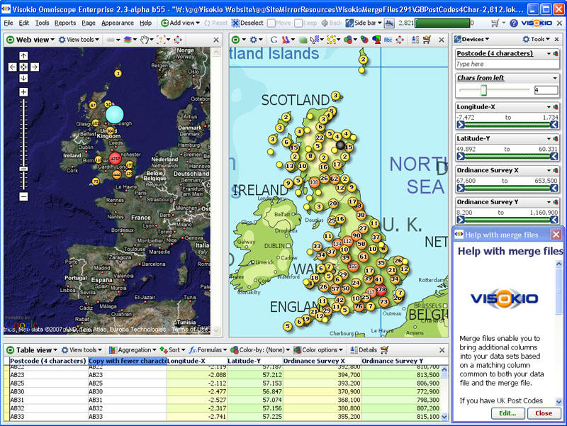 [368] [368](click for larger image) |
Use this free merge file to add decimal longitude and latitude columns corresponding to the centres of British 4-character Post Codes, plus 6-digit British Ordinance Survey coordinates, to your files. This file can also be used to add Post Codes to files containing Ordinance Survey coordinates. Instructions and links to further help are contained in the file. Note: a full character UK post code file is available from the DataManager workspace Lookup data menu (2.6+) |
|
Use this free merge file to add decimal longitude and latitude columns corresponding to the centres of 42,192 5-digit Zip Code districts, including those located outside the 50 States. Contains two formats, 5 digits of zero-padded text, and unpadded integer numbers (up to 5 places). Instructions and links to further help are contained in the file. |
| France | French Post Codes Merge File [372] (IOK) 127 KB | |
| Germany | German Post Codes Merge File [373](IOK) 183 KB | |
| Italy | Italian Post Codes Merge File [374] (IOK) 122 KB | |
| Belgium | Belgian Post Codes Merge File [375] (IOK) 32 KB | |
| Denmark | Danish Post Codes Merge File [376] (IOK) 20 KB | |
| Switzerland | Swiss Post Codes Merge File [377] (IOK) 63 KB | |
| Australia | Australian Post Codes Merge File [378] (IOK) 71 KB | |
| Canada | Canadian Post Codes Merge File [379] (IOK) 43 KB | |
| Spain | ||
Use the above free merge files to add map coordinates based on post code fields (columns) in your data. Other country files are available... if you need another country, please contact us. [86] For a list of available Maps, see our Maps Library [48].
Omniscope Web Views can be used to display context-sensitive notices or adverts on tabs within files, assuming the user is online. This can be used to generate analytics data on usage of each tab.
Omniscope Professional and Enterprise Editions allow you to create Omniscope files that display banner adverts with live links to the advertiser on each page. The banner adverts can be positioned at the top, right, left or bottom of the display. Currently, you can specify only one banner image per file (rather than per page), and one link per image, although this will change in future versions.
In general, rectangular images look best, such as typical full-width banner ads, displayed either vertically at the sides:
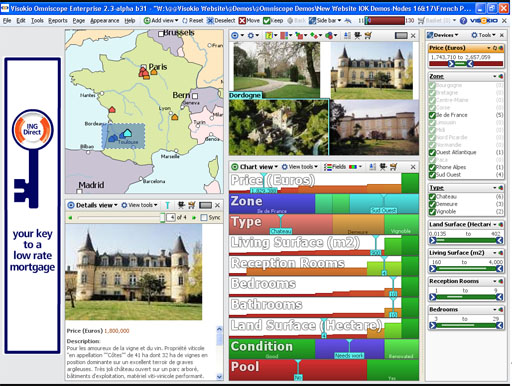
... or horizontally at the top or bottom:
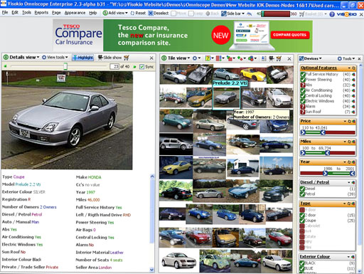
,
The user guide has been replaced by the video tutorials [1] and the remaining pages are being migrated into the knowledgebase. Please bear with us as we remove and rearrange these remaining pages.
The contents of this User Guide are searchable and navigable using either the links below or by using the left-hand User Guide navigational menu. You can use the custom search field at the top right of any page to enter specific commands, terms or phrases and find all references in the Forums [380], this User Guide, and the KnowledgeBase [381] (which contains moretechnical articles of potential interest to IT support and DBAs/developers).
For a printed version of the entire User Guide or any section, click on ‘printer friendly version’ at the bottom of the first page you wish to print, then use your browser Print function. If available, choose 'PDF' as the printer from your browser to obtain a PDF file version. Alternatively, you can download the prepared PDF files posted here, although they will not aways contain the very latest version of all the pages.
![]() Printable User Guide [382]
Printable User Guide [382] ![]() User Guide (PDF) [383] (21 MB)
User Guide (PDF) [383] (21 MB) ![]() Training Guide [384](PDF)
Training Guide [384](PDF)
Overview [386] - this is a simple, one-page overview of key Omniscope functionality illustrating typical tasks in 10 steps; install Omniscope, prepare data, load/import data from a spreadsheet, check the data types, explore/check the data, display the details, add/change views, create report tabs, add links, and save the configured Omniscope files for distribution to others.
Installation [387] - describes the Omniscope installation process on Windows. Details regarding non-Windows installations, rollouts to administered desktops and network installation options, etc. are covered in the KnowledgeBase [381].
Activation and de-activation [388] - illustrates how to activate new installs, refresh activation for version upgrades, and de-activate prior to re-building or moving machines.
Welcome Screen [389] - if no data file is open, branded Omniscope installs display a welcome screen with useful links to learning resources and other settings.
Demo files [390] - every installation contains many fully-configured demonstration files illustrating key features and uses of Omniscope. Consult this page to lfind links to more detailed or specialised demos most relevant to your own data sets and intended uses. See also Case Studies
Training Guide [384] - recommended 6-phase approach with printable checklists outlining the sequence of specific 'best-practise' steps in detail. Print this section and follow the checklists. Downloadable versions are available for use as outlines for structuring training sessions.
The free Viewer enables navigation, filtering and printing using Omniscope files prepared by others, including the demo files included with Omniscope. You can display or send this direct link to this chapter to your file recipients together with your IOK files: http://www.visokio.com/using-viewer [391]
Viewer Main Toolbar [392] - introduces revealing and using the navigational icons/buttons available on the Main Toolbar, which may be hidden (or in some cases displayed on the Sidebar) on some tabs of the files you receive.
Using the Sidebar(s) [393] - covers the basics of selecting and filtering using the Sidebar(s) which are usually displayed on most tabs of the files you receive.
Tabs and Views [394] - navigating presentation/report tabs and using views for filtering and producing screenshots and printed views.
Welcome Screen [395] - closing a file in the free Viewer reveals the Welcome Screen, from which other files and features can be accessed. This screen is not displayed when deploying files using Omniscope Online and the unbranded version of the free Viewer.
Printing [24] - Omniscope can print static images of views, single or multiple tabs, to a printer or in common file formats like PDF and PowerPoint
Using Omniscope Online [396] - Omniscope Online is a version of the free Viewer that can be deployed from a link in a web page to users' machines using Java Web Start technology. Both branded and unbranded versions of the free Viewer are available, although use of the unbranded version requires the Enterprise Server Commercial Publisher.
DataManager [398] (2.6+) - the DataManager workspace is a highly-visual drag and drop interface for defining import, assembly, transformation and various output and distribution options as repeatable flows with defined data refresh options.
New file [399] - Populating your own small file by typing in imaginary (or real) data is an excellent way to get started with Omniscope. Open blank table and type or cut-paste data into cells. You can also cut-paste tabular data sets from documents or web pages to provide a starting point.
Open file [400] - importing data from spreadsheets and other types of data files, maintaining links to source data
Open map [401] - introduces the Map View and various ways of adding maps and geographic coordinates to your data sets.
Database connections [402] - Using either ODBC or JDBC protocols, Omniscope can establish and refresh direct connections to relational database tables and reporting views using the Database Connection Wizard wizard, which can import the results of any SQL statement that returns a table.
Connectors [403] - connectors enable data import, refresh and synchronise features for data hosted on popular remote 'cloud computing' SaaS platforms, including e-mail folders, collaborative online data services like Google spreadsheets, general-purpose application platforms like Salesforce/Force.com, free information sources like Google Analytics as well as traditional subscription data 'feeds' like Bloomberg.There are also options to gather data about folders of files on your network, and import/export image collections in Omniscope file format. Click on the links below for more detailed sections on each connector.
Bloomberg Connector [404] E-mail Connector (POP3, IMAP) [405] Google Spreadsheets [406] | Facebook [407] Google Analytics [408] Website Mapper [409] | Salesforce Connector [410] Open folder of files [411] Open image set [412] |
Merge data [413] - the Merge Data wizard makes it easy for anyone to assemble and update data sets from disparate sources. An Omniscope can have any number of files as sources, and all merges are repeated on every refresh.
Adding Images [414] - Explains the process for associating folders of images (image sets) with your files and referencing them for display in various views. Omniscope can associate more than one image with each record (row), and can associate more than one image set with a file, either embedded or for delivery via the web. If multiple images are available for some records, slide show mode can display a sequence of these images for each record selected.
Refresh options [415] - explains options for refreshing data from linked sources, including the Automatic refresh option, and how to unlink and re-link Omniscope files from/to source data files, including other Omniscope files. Using Omniscope IOK files as 'datamart' source files permits many 'personalised' Omniscope files to be distributed and auto-refreshed from the same central Omniscope file, itself typically being refreshed more frequently on the server from the data warehouse.
Editing Cell Values [417] - the Table View permits you to edit values in data sets at individual cell, value or column level using familiar keyboard shortcut commands
Rows & Columns [418] - adding and deleting rows and columns, setting column orders, configuring row height etc.
Dates & times [110] - specifying and changing the format of data stored in your source files as imported Omniscope date & time values.
Tokenized data [419] - use this data sub-type option when you need more than one value/image in the same cell of a given row, i.e. to enable filtering with one-to-many relationships in 'flat' data sets, or to display multiple images per row of data.
Time Series [420]- Omniscope stores repeated observations over time as rows (not columns). Consult this section if you plan to create time-series displays from your data set.
De/Re-pivot [421] - Omniscope includes powerful functions for changing the orientation of data in the files, such that rows become columns, or columns become rows.
Edit/Add Map Coordinates [422]- Omniscope enables you to add or edit geographic coordinates associated with a map manually. Use this approach to check your geographic coordinates, add missing coordinates, and refine the coordinate columns in your data set by referencing highly detailed online mapping resources
Data entry - see the Details View [20] to learn how this view can be configured as a data entry screen that can be displayed on any tab.
Omniscope enables you to define evaluated Formula fields (columns) which calculate the values to display using the values in other fields (columns). Omniscope formulae can also incorporate variables, user-defined ranges of assumed values specified in terms of maximum, minimum and default values. Formula fields are defined using standard functions using the same syntax as for Excel. Functions available for use in constructing formulae include a library of special Omniscope SUBSET and older DATASET functions that operate across one or more entire columns of data sets. Example formulae useful for accomplishing common tasks are also illustrated in this section.
Provides detail on configuring the filter/query devices displayed on the Side Bars with the Devices and Tools Side Bar drop-down menus, using the functions available on the filter/query devices, and the commands accessible by right-clicking on the devices.
View Details [23] - Explains the options for displaying some or all the values associated with individual records or selected groups of records - the Details pop-window, the Side Bar details display options and the Details View. The highlighting function, which shows the position of selected records in all open views, is explained and illustrated. Automatic record cycling and slide show image displays that provide file recipients with automatic, unattended 'tours' of the data are also covered.
Aggregating Data [425] - most Omniscope View Toolbars include an Aggregation drop-down dialog which enables you to define an aggregated transformation of the underlying granular data set, and also define the aggregation functions to be applied across the aggregated values in each field (column). Each view on any given tab can use a different aggregated view as defined by the settings on each View Toolbar Aggregation drop-down
Guide to Views [21] - details the commands and options available for each of the different views in Omniscope. Visit the top page, or lick the links below to go directly to the section relating to a specific view. View Toolbar commands common to most Views are documented here.
|
Adding Links [429] - Explains the process for adding local links, using pre-configured links to free web services and creating custom web links launched by clicking on specific cells/values in your files.
Adding & Styling Text [431] - Free-form text, links, and images not in the data set can be added to Report files as text tabs, and can be added to any view tabs as Titles and Annotations. Explanitory text can also can be added to views windows by editing view headers and displaying view footers. Any number of Content Views can be added to any tab and sized to complement the other views. Each Content View can contain styled text, links, images and formula-driven dynamic text.
Managing Layouts [432] -
Edit Layout Modes [433] -
Using Styles [434] -
Create Reports [435] - Introduces the process of creating and modifying Reports Pages, the Reports Navigator, the importance of committing or reverting changes to Report Pages, how to exit Reports Mode and using various menus for managing all the Report Pages already configured in a given file.
File Appearance [436] - Highlights a few of the more commonly used options for branding the overall appearance of a given file using Cover and Back information pages together with your own corner logos, etc. Options for adding your corporate identity to installations of Omniscope itself, simplifying display menus, and adding banner advertising displays to Omniscope files are also referenced.
Creating DataPlayers [437] - DataPlayers are exportable, data-bearing, interactive Flash 'dashboard' .SWF files which can be created, refreshed and exported from Omniscope to web pages and documents such as PowerPoint, Excel, PDF ...with full interactivity. This section explains how to create, combine and export many different, highly-configurable DataPlayer view types using the DataPlayer View of Omniscope.
File Security Options [439] - Omniscope files can be saved with extensive file security options controlling who can open Omniscope files, for how long and under what circumstances. 'Layered' security options are available for securing data against unauthorised copying (not even cut-and-paste) and for implementing highly-secure deployment options such as domain locking and/or 'walled gardens'.
Commands Reference [440] - summarises the Main Toolbar command menus and provides links to documentation for current and previous versions. Use the links below to go directly to the command menu of interest.
Main Toolbar [441]- documents the icons and options located in most Layout modes on the Main Toolbar to the right of the command menus.
Version 2.5: | File [442] | Data [443] | Tab [444] | Layout [25]| Toolbars [445]| Settings [446]| Help [447] |
(click links above to go directly to the Commands Reference page)
Welcome to Omniscope! This section covers the basics of Omniscope, and provides links to more detailed sections located elsewhere in this User Guide and our KnowledgeBase [381], which contains more depth of technical articles and worked examples. The Training Guide [384] at the end of this section provides a phased, step-by-step 'roadmap' to fully configuring any Omniscope file, with detailed checklists you can print and follow as you work through your files.
Overview [386] - a one-page general introduction to the process of using Omniscope.
Installation [387] - This page covers installation on machines running the Micrsoft Windows operating system. If you are installing from a Mac, the Mac version will be preselected and you should follow the instructions that appear on the download page. There are currently some Mac version limitations [449]. To use with Linux/Unix, an experimental JAR-only version of the free Viewer is available. Choose "Linux / JAR-only" on the download [450] page, and see Command Line [451] for more information on using this. More detailled information on installing on other operating systems (Mac, Linux, etc.) is in the KnowledgeBase [452].
Activation & De-activation [388] - describes the process for activating (new installations), refreshing (version upgrades) and deactivating Omniscope installations prior to re-building or moving machines.
Welcome Screen [389] - the Welcome Screen opens before any file is loaded, with shortcuts to frequently-used commands, recently opened files, links to demos and links to learning resources. Note: The Welcome Screen will look different in free Viewers [391] than it does in activated editions used to import/edit data and configure files.
Opening demo files [390] - opening the demo files included with Omniscope is a very good way to learn what is possible. During your free trial, you can export the underlying data then try re-configuring the file to match the demo. Additional online demos are here [453].
Training Guide [384] - start by following this 6 phase, step-by-step detailed checklist approach to importing data, configuring views, creating a presentation and sharing it with others.
Omniscope free Viewer will open any Omniscope .IOK file of any size, up to the limits of your PC [454]. Each new Viewer installation also includes a free 30-day trial of Omniscope Professional. During the 30-day trial period, you can import your own data from spreadsheets and databases, and you can export data from any of the embedded or online demos as spreadsheet files to see how these files were configured from tabular data. You can also use the DataPlayer View to create exportable, interactive Flash DataPlayers for embedding in web-based 'dashboards' and common documents like PowerPoint, Excel and Adobe Acrobat .PDF. After the 30 day free trial expires, the installatation reverts to being a free Viewer, so there is never a need to un-install.
If you don't yet have Omniscope installed, install the free Viewer [450]. The installation sequence (for Windows) is shown here [387].
You can open tabular data sets such as spreadsheet files directly in Omniscope. A sample 6-column .CSV file for use with this Quick Start page is attached here [455]. Download the sample data file, or choose a different file containing your own data. Try to avoid any blank rows, formatting and merged cells in your source spreadsheet file. Check that your spreadsheet looks like this. [456]
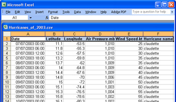 |  |
During your 30-day trial period, or if you are already running an activated Edition, you can open any of the demo files and use File > Export > Export files and select the Data tab to save the data as a CSV or other supported file type. You can then re-import the data using File > Open file [400], and compare with the embedded demo to see how the demo file looked before it was configured. For more detail, see the section on Importing Data [397].
Omniscope will open the file displaying three default views; a Table View, a Chart View and a Pie View, as well as the right Sidebar, with various filter devices created by default.
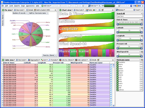
The Table View is most familiar, but the Chart View is very useful for gaining insight into the structure of the data set at a glance.
Omniscope examines the data in each column and makes some assumptions about the column's data type, which are not always optimal. When importing data for the first time, always check and (if required) modify the data typing (i.e. whether a column's data is typed Numbers, Dates and Times or Text). If there are only a limited number of different Text values, Omniscope will usually type the data as Category. To review and edit data typing, click on Data > Manage Fields [31].
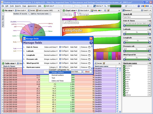
Frequently, Omniscope assumes that identifying numbers should be treated as integer numbers. You should change the data type of all-numeric reference identifiers to 'Text'. Remove the separators in the number before converting to text using Options > Formatting options: {untick} Show thousands separator. Also, for some date and time fields you may be asked to clarify the date/time format used in your data before Omniscope can recognise it accurately as dates and times. For more detail on data typing options see Data > Manage Fields [31].
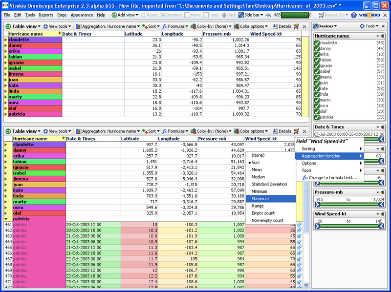 [457]
[457]
Using the hurricane example file, close the Pie and Chart Views, and open a Table View. Click on the Aggregation command to aggregate all the observations over time by Hurricane Name. By default, all of the columns will show the sum of the observations, nonsensical in this case. Right-click on each column header, choose Aggregation function and display the median for the Longitude and Latitude columns, the mean (average) Pressure and the maximum Wind Speed. The example above shows two Table Views, the lower with the aggregation functions defaulting to Sum, and the upper showing the same data with the view configured to show meaningful results that can be used to spot errors in the data. From version 2.4, the Aggregation drop down menu on the View Tolbar can be used to set both the fields to aggregate on and the aggregation functions to apply to visible columns in the aggregated view.
For more detail, see Using the Table View [3]
Next open only the Chart View, which provides a horiziontal overview of all the columns in the data set. In the Chart View, under View Tools > All charts, for each field (column) name you can decide how to graph the values in each column, e.g. histogram bars, pie charts, statistical summaries, etc. Use this analytical view to further scrub your data.
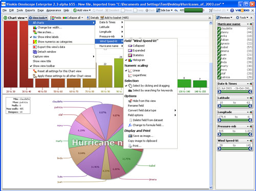
The right-click menu provides links to many other settings related to the selected field (column). You can re-order or hide fields that are not required by dragging or unticking them in the Fields drop-down pick list.
For more detail see Using the Chart View [4]
To see the values of all the fields for a given record (row), in the Table View, double-click on the record (row) header (farthest left). A configurable Details pop-up window appears, showing the values for the selected record. You can configure the Details pop-up window extensively using the Configure menu.
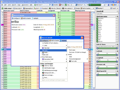
Omniscope has 12 different views that can be used to visualise and explore your data. Click on ![]() Add View in the Main Toolbar and try each of the views not already showing. Each view has its own Toolbar and pick lists for selecting which fields (columns) to display. The powerful Bar View has a tab that you pull from the left side to reveal all the options. When you have finished with a view window, click on the [X] in the upper right hand corner to close it.
Add View in the Main Toolbar and try each of the views not already showing. Each view has its own Toolbar and pick lists for selecting which fields (columns) to display. The powerful Bar View has a tab that you pull from the left side to reveal all the options. When you have finished with a view window, click on the [X] in the upper right hand corner to close it.
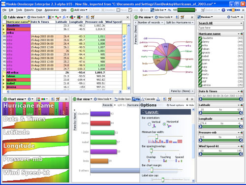
All users of your Omniscope file are not expected to know how to open views, set multiple filters etc. Instead, you decide the most important combinations of views, filter settings and messages to other users, and save them as persistent tabs, which can be considered report pages or simply separate workspaces. Tabs are preconfigured combinations of views, filter settings, formula variables and annotations. If you save an .IOK file in Reports Mode with a Report Page selected, it will open and navigate just like a slide show presentation.
To create a tab in your file, click on Tab > New > From current layout from the Main Toolbar.
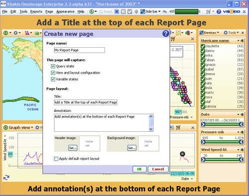
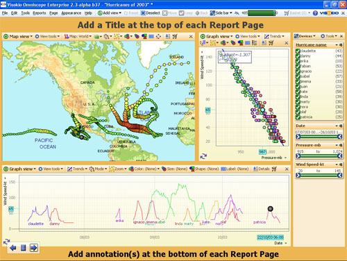
If you make further changes to a tab, always remember to click Commit to make them lasting. If you do not wish to change a tab after performing some operations on it, click Revert to return the Report Page to its configuration when you last committed or created it. This is useful when giving live presentations. There is also an optional floating tab navigator in the lower left-hand corner, which reveals itself when you hover your mouse (Toolbars > Floating tab navigator). For more detail, see Creating and Managing Report Pages [435].
Omniscope integrates with the Web by incorporating defined links based on your data. Values in your data are automatically transformed into links when users of your files click to display related web pages. The web pages can display either in the Web View of Omniscope, or the users' default web browser. To configure your own web links or add links to local documents on your network, use the Add links wizard available from Settings > Links > Add web or Add local link.
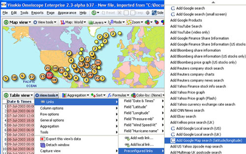
Omniscope also includes pre-configured links to popular, free web services that accept a single string of text as an input, such a Google, EBay or Wikipedia searches, or financial data on specific securities from Bloomberg, Reuters, Yahoo etc. Select Settings > Links > Preconfigured links to see the menu of currently available free web services.
Once configured, save your Omniscope file using various options for distribution. Go to File > Save As and you will be presented with the Data Export wizard set to save your file as IOK files. This wizard offers many options to save all or only selected subsets of your fields and/or records, plus the option to set file update/refresh options, and to protect your data from unauthorised access and copying.
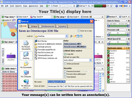
There is a single installer file for all Editions available from our downloads page. [450]
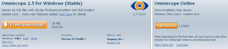
Full - the first time you install Omniscope, you will be offered the full installer, which includes a full version of Java that will be installed as the private virtual machine (PVM) together with Omniscope. If you update a beta version of Omniscope frequently, you can update your installation using the much smaller Light installer. However, due to bugs in Java being fixed all the time, it's best to download a full version of Omniscope, with the latest version of Java, at least once per month.
64-bit - If you are using a 64-bit operating system, make sure to download the 64-bit version of the installer. More on 64-bit operation. [458]
Omniscope Online - if you are on a machine that does not allow you to install Omniscope, you can still download the free Viewer from the Launch link, and use it to explore the demo files and other IOK files you may have received. More on using Omniscope Online [396].
Omniscope is a standalone installed application requiring administrative privileges to install. There is only one installer file to download for all Editions of Omniscope. The installer includes a 30-day free trial of Omniscope Professional. On expiry of the initial 30-day trial, the installation will revert to a free Viewer, which never expires. There is never any need to uninstall.
To install on Windows, visit our download page [450]and click on the Free Download orange colour button. If you are installing on a 64-bit machine, make sure to select the 64 bit installer. Use the full installer the first time you install, but you can later choose 'lightweight' installer to speed download times.
1.) Click "Run" or "Save" when prompted. 2.) If you choose "Run", the installer wizard will launch automatically. 3.) If you choose "Save", the installer file OmniscopeOfflineInstaller.exe will be saved. if you choose "Save", 4.) Find the file "OmniscopeOfflineInstaller.exe" file (icon shown right) and double-click to launch the installer wizard. |  |
When the installer is started you will see Vista User Account Control prompt: "Program needs your permission to continue". Click Continue to proceed. Please note that if you are not logged in with Administrator privileges on the machine, you will need someone with an Administrator account to install Omniscope. This will change in version 2.6.
The next screen is the set-up wizard, click Next >
The next screen asks you to accept our licensing agreement. More information on the terms of our licensing is available here [459]. Tick the "I accept the terms of the License Agreement" box and the Next > button to continue.
You will see an installation progress bar, a list of files being installed and then this screen: Click Finish.
Unless you have previously licensed Omniscope, your installation will open as a free Viewer, allowing you to open and navigate any Omniscope .IOK file, such as the many embedded and online demos. [453] In addition, all free Viewer installations come with a free 30-day trial of Omniscope Professional, enabling you to make files with your own data. At the end of the trial period, unless activated the installation reverts to a general-purpose free Viewer...no need to uninstall.

By default, Omniscope installs with the option to automatically check for updates ticked. Test that you have the latest version, and that your automatic update function is working by clicking Help > Check for software updates now...
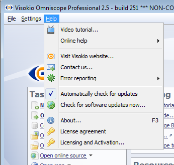
If you have a problem contacting our update server, it may be that your machine is accessing the Internet via another machine known as a 'proxy server'. Due to limitations in Java, Omniscope is sometimes not able to detect these settings automatically. They useful not just for updates, but also for Activation, bug reporting, etc.
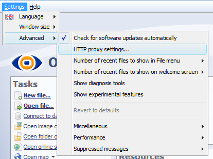
If your organisation is using a proxy server, you may need to ring your support person or network administrator to discover the settings Omniscope needs.
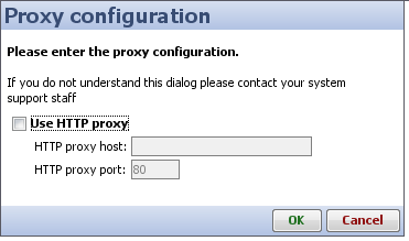 [460]
[460]
More information on Proxy Settings [461].
If you intend to install an Enterprise Edition with automated Scheduler and Generator capabilities, make sure to install on a machine that will not be turned off, and activate the installation from an account that will not log-off. See the Automation [462] section of the KnowledgeBase for more information on installing an Enterprise Edition as a Windows Service [463] to provide always-on data refresh and other automation services.
Omniscope opens to display the Welcome Screen with shortcuts to frequently-used commands, recently opened files, links to demos and links to learning resources.
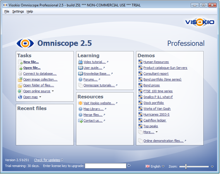
TasksThese commands are also on the File menu on the Main Toolbar, but can be used from the Welcome Screen for connecting directly to sources of data (including online data sources, images and maps) which are not already in an Omniscope file. | LearningLinks under this heading point to various resources for learning more about how to use Omniscope. | DemosOmniscope is completely general-purpose. Embedded demos provide working examples of how to use Omniscope to make the most of your data. A wide range of examples are provided drawn from a cross section of typical uses. | ||
Recent filesDisplays the files you have open most recently. Clicking on these links will open the file, provided the file name and location have not changed. | ResourcesLinks under this heading direct you toward potentially useful sources of information, maps and data you may wish to add to your files.
| |||
ActivationYour version/build number is displayed at bottom left, and you can click 'Check for updates' to ensure that you have the latest build for your version. If you are unactivated and still in your 30-day trial period, a link is displayed for you to contact us for a formal trial key, or an Enterprise trial key. Once you have a key, you can activate by entering it in the text box. | LanguagesChoose the language you want Omniscope to display in commands menus and dialog. Languages displayed in violet are less than 90% complete. Anyone can add a new translation or improve/localise an existing one using Omniscope as explained here [465].
| ZoomKnown as screen resolution in earlier versions, Zoom allows you to magnify or reduce the entire Omniscope interface to make text and buttons larger or smaller. Use Zoom to increase the readability of text on a high-resolution screen, or reduce the size of buttons on low-resolution screens. Zoom can improve legibility of printed output and is also useful for the visually impaired. |
![]() When you have a file open, you can still zoom in and out by clicking on the Zoom icon/drop-down in the Main Toolbar of the application. You can also revert back to the default settings by clicking on the Revert to default option which is located under the slider. This option is also available from the Welcome Screen by clicking on the small black triangle right of the zoom slider in the bottom right hand corner.
When you have a file open, you can still zoom in and out by clicking on the Zoom icon/drop-down in the Main Toolbar of the application. You can also revert back to the default settings by clicking on the Revert to default option which is located under the slider. This option is also available from the Welcome Screen by clicking on the small black triangle right of the zoom slider in the bottom right hand corner.
Full working examples showing the many features of Omniscope are available either from File > Open demo or the Welcome Screen [389]. During your free trial, you can try exporting the underlying data sets as CSV spreadsheet files using File > Export > Export file {Data} dialog, then using File > Open file to import the exported data set and configure it to match the original demo file.
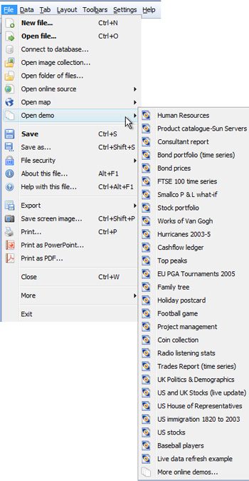 | Human resources - a very comprehensive demo file based on a typical company staff. Every record (row) is a person, with images, a position in an organisational hierarchy, and an office location for mapping. Includes multi-variate simulation modelling of salary increase options and an alerts dashboard. |
Anyone can configure Omniscope files systematically following the 6-phase checklists outlined below. Most issues in configuring Omniscope files arise because essential steps like changing default data typing assigned on data import are not addressed BEFORE moving on to other tasks. Following the checklists below, anyone can achieve rapid, reliable results and make best use of Omniscope. This phased outline and checklists also serve as a useful guide for structuring training sessions.
Options for importing data into Omniscope include importing from delimited data files like CSV and XLS, relational tables/reporting views created using SQL statements that return a table, various remote-hosted or 'cloud' based data sources via connectors, transformed tabular XML [472] and some multi-dimensional 'cube' data structures (Data Manager Edition only). The Enterprise and Data Manager Editions (2.6+) has a dedicated visual drag and drop data assembly, filtering and transformation Data Manager [398] workspace that can be used independently of Omniscope. The Professional Edition has Most of the options are documented in the Importing Data [397] chapter of this User Guide, which includes sectons on creating [399]and importing data files [400], making and refreshing database connections [402], using connectors [403] to online/remote data sources and more. More technical articles and examples relating to importing data via Data Manager or the Professional EDition Data Import and Merge Wizards are available in the KnowledgeBase [381], which includes sections on supported data file formats [473], examples of database connections [474] using ODBC and JDBC, and other related topics.
This checklist covers tasks you should perform AFTER importing a starting data set for the first time, but BEFORE beginning to analyse how to filter, visualise or present the complete data set. Most of these tasks are coved in the Editing Data [416] and Managing Data [423] chapters of the User Guide.
The Data Management phase focuses on data set completeness and correctness. Data typing assumptions made by Omniscope on import should be checked, columns duplicated, expanded, collapsed or tokenized to facilitate end-user interaction with your file. In this phase, 'data scrubbing' view configurations (rather than final presentational views and layouts) are used, normally working on a single tab entitled 'Data Set' or similar. Use Table View column sorting and the Chart View to examine extreme values in each column, correct null (blank) and missing values, and add related content to the file, such as image sets, maps and links to related web pages and web services.
At the end of this phase, the single 'DataSet' tab should reveal all non-empty and non-uniform data fields and filters, using both Sidebars if necessary to check all the filter devices in the Table/Chart View(s) without aggregations or groupings. You may need to duplicate certain columns so that they can be typed or formatted differently, providing different filtering options for users. Note: it is good practise to always leave this unfiltered 'Data Set' tab accessible as the final tab on the far right of the file tab set, providing an instant, credibility-enhancing maximum granularity view of the data to any user who clicks on the tab.
This phase focuses on optimising the data set for its intended audience. The checklist covers tasks you should perform, or options you should consider AFTER you have imported/merged all the data sources and 'scrubbed' the data to ensure correctness and completeness, but BEFORE you begin to define the best ways to visualise and present the data set as a presentation or reporting 'dashboard' file. Most of these tasks are covered in the Managing Data [423] and Configuring Files [475] chapters of this User Guide.
In this phase, column re-naming should be used to shorten names to save space and make them instantly meaningful to the end-user audience. Unneeded columns (especially empty or uniform-value columns) can be hidden or deleted, and the number of unique category values can be reduced, either via re-naming/consolidating values with data edits, or by adding formula columns that re-categorise records into fewer categories. Formulae can also be defined to transform imported data fields into more useful values and to detect alert conditions to be highlighted. If you use formulae to convert/reduce total category values, or to extract useful data fields from within text strings, your changes will be re-evaluated on every refresh. Aggregations can be set and aggregation formulae specified to create transformed views of the data for use with most views.
At the end of this phase, all the data, images, maps and link references required to meet end-users' requirements should be in the file, and the single 'Data Set' tab should show all the fields, both data and formula, which have not been globally hidden. Additional 'Subset', 'Formula' and 'Aggregated' tabs will have been added to show useful data subsets made reference-able as Named Queries, the inputs and results from defined Formulae, and various Aggregation settings with key values calculated according to specified aggregation functions displayed. Don't worry, you will delete all these preliminary testing tabs by the end of the next phase.
This checklist covers tasks your should perform, or options you should consider, AFTER you have optimised your data set, defined reference-able data subsets i.e. Named Queries, added Formula fields that calculate useful values and alert conditions, and defined useful Aggregation settings (including aggregation functions by field/column), but BEFORE you decide the optimal combinations of views that best suit the requirements of the file. Most of the documentation of the Views and how each is best used is in the Exploring Data [424] chapter of the User Guide.
Omniscope offers a large and growing number of views, each of which is highly configurable. In the Visualisation phase, you test each View on its own tab, seeking the best configuration(s) of each view for the data set and the requirements of your intended audience. You may create more than one variant of each view. Views determined to be of limited value to the audience can be hidden.
At the end of this phase, you should have a tab for each view you plan to use, with one or more variations of the view on each tab, perhaps some displaying subsets of the data defined by Named Queries, and others displaying Aggregated views with column-specific functions as defined in the Aggregation settings in each view.
This checklist covers tasks your should perform, or options you should consider, AFTER you have defined the views you plan to use, but BEFORE you create the tab sequence that will convert your file into a final presentation. Most of these tasks in this phase are documented in the Reports & Presentations [430] chapter of the User Guide.
Unlike previous phases, the Presentation phase takes a minimalist, 'zero-based' approach to file configuration, i.e. the bias is that everything should be hidden unless it is needed on a specific tab to make a specific point or enable a particular end-user interaction. Working with the most useful view configurations created in the previous phase, the objective of this phase is to create a multi-tabbed presentation where each tab is addressed to a specific issue with a specific message supported by the data. In this phase the philosophy is "less is more" to simplify the audience experience, but with credibility-building granular detail always only one click away. Don't be afraid to create many different tabs, each focused on specific user groups and points to be made, rather than trying to put too much on one tab. The objective is to create a file that opens and navigates just like a slide presentation.
At the end of this phase, you should have a highly-visual, interactive, multi-tabbed presentation file that your users can quickly and easily consult, filter, and print.
This checklist covers the final file configuration options relating to branding, data refresh and how others will be able to use the file. Most of the tasks in this phase are documented in the Save & Export Files [438] chapter of the User Guide.
In this phase, Help screens are added, along with selected branding options (opening screen, closing screen, banner ads, corner logos, etc.). File settings relating to refresh, file security, and other publishing options configured in the file when saved are all considered in this final phase.
The Data Import phase is documented primarily in the Importing Data [397] sections of this User Guide, which includes topics such as importing data files [400], making and refreshing database connections [402], and using connectors [403] to online/remote sources and more. More technical articles and examples are available in the KnowledgeBase [381], which includes sections on supported data file formats [473], examples of database connections [474] using ODBC and JDBC and other related topics, such as importing transformed XML. [472]
Getting started with Omniscope usually involves importing a copy of a structured table of data, such as a spreadsheet file or a reporting view from a SQL-based relational database. Options include:
1-01 Create new file [399] - manually type or cut and paste data into a blank Omniscope file
1-02 Open data file [400] - import data from a delimited data file (see potential issues list below)
1-03 Connect to database [402] - connect to a relational database using ODBC or JDBC protocols
1-04 Using Connectors [403] - use one of the available Connectors to access/import remote-hosted data
1-05 Open image collection [412] - open and import a folder of images, together with user-editable tags
1-06 Folder of files [411] - access and analyse a folder of files (documents, audio/visual media, etc.) to create a data set of filenames/paths and user-editable tag names
1-07 Open map [401] - access our Map Library [56], download a geo-coded map file and build a data set, including manual or automatic placement of records by decimal longitude/latitude. Alternatively, screenshot an online map image, note some reference coordinates, then use Omniscope to geo-code the image and build a data set to overlay the image map.
1-08 Perform merges [413] - Use the Merge Wizard if additional data from other sources needs to be joined or concatenated with your initial data set. Before performing a join, test the uniqueness of join criteria columns using the Table View: View Tools > Tools > Select duplicate records command.
Note: If new, currently unspecified columns might be added to one or more of your merge files in future, do not specify the fields to import, so that Omniscope will continue to import all fields in future. You can then Hide or Delete any unneeded fields as a remembered action.
Data files are often not delivered formatted according to precise international standards. Differences in formatting of data within tables and delimted files around the world can affect data import and display in Omniscope. Below are some common issues which you may encounter when importing data tables into in Omniscope:
Regional formatting - When importing data by opening a CSV or Excel XLS file, Omniscope analyses the data in the file to determine how the data is arranged and which fields (columns) are most likely of data type Text, Numbers, or Dates & Times. The regional settings in your computer's operating system (Windows, or Mac, etc.) have a strong influence on this operation. For some combinations of settings and data formats, Omniscope cannot reliably detect the situation automatically. If your data opens incorrectly and your fields are not correctly structured, numbers have the wrong decimal place, etc. please consult the File > Open file [400] dialog page, which contains options to help with these situations.
For example, if you know your data has been formatted for a different region, change the Locale drop-down accordingly. For example, if you live in Germany but have received a CSV from an American customer, you should choose "English (US)". If you find Omniscope gets things wrong and your data is incorrectly recognised, you can disable auto-detection of dates and numbers by deselecting the two Recognise... check boxes on the File > Open file [400]dialog. All fields will open as Category or Text data and their text values will be preserved. You can then use Data > Manage fields [31] [35]to configure each field (column) as you would like it to display.
Data file delimiters - CSV stands for "Comma Separated Values", which means the cells in each record (row) of the data table are separated by the comma character. However, this is not a formally-documented standard, and if you are in a region that also uses the comma in numbers instead of the decimal point (e.g. several European countries, such as France), some versions of Excel create CSV files that use a semicolon as the separator character. Sometimes these multi-column tables files are saved with a CSV or even a TXT extension. Omniscope is unable to detect this situation automatically. If you open such a file in Omniscope, your data will very clearly be wrong, with most columns appearing as text with semicolons. To avoid this problem, use the File > Open file [400]Customise data import dialog to change the separator character to a semicolon " ; ". You can also do this with 'pipe' "|" delimited files, but you must first change the file extension on the data file to .CSV, even though the file is really is 'pipe' and not comma delimited.
Dates & numbers - If you are running on Windows, when importing data that is in a delimited text format such as Excel XLS, CSV or TSV (tab-separated values), Omniscope will use your Windows Regional Settings to try to automatically recognise data. For example, for a PC with United States Regional Settings, Omniscope will recognise "5/13/2005" as a date and "1,500.5" as a number. For some international users, however, this may not work as expected and the result will be an import of all columns as data type Text (shown in Omniscope either as multi-coloured Category columns or white Text columns). If this occurs, you can usually manually convert fields (columns) containing numbers or dates and times using the Data > Manage fields [31]dialog. For more information on formatting dates and times and managing time zones, see the section on Dates & Times [110].
Go to Data Management Phase [467]
This checklist covers tasks you should perform AFTER importing a data set (or merging in another) for the first time, but BEFORE adding further content or beginning to analyse how to filter, visualise or present the data.
The Data Management phase focuses on data set completeness and correctness. Data typing assumptions made by Omniscope on import should be checked, columns duplicated, expanded, collapsed or tokenized to facilitate end-user interaction with your file. In this phase, 'data scrubbing' view configurations (rather than final presentational views and layouts) are used, normally working on a single tab entitled 'Data Set' or similar. Use Table View column sorting and the Chart View to examine extreme values in each column, correct null (blank) and missing values, and add related content to the file, such as image sets, maps and links to related web pages and web services.
Using the X in the upper right-hand corner, close all the default opening Views on the opening Tab, except for the Table View [3].
2-01 Check data typing [31] - On import, Omniscope assigns a data typing assumptions to each column in the data set: 'Text', 'Numeric' or 'Date & Time'. If the number of unique text values in a column is less than a defined threshold, the field will be further typed 'Category'. Sometimes, columns of identification numbers which are not used in calculations and usually searched as Text are mistakenly typed 'Integer Number' with separators added. Data typing can be reviewed and changed using the Data > Manage fields [31] dialog. Make sure to remove the separators from numbers before changing them to text by unticking Data > Manage fields > {column} Options > Show thousands separator. Ensure that data which is stored in the source file as a valid data and time has been recogised and imported as Date and Time rather than Text, as discussed here [110].
2-02 Set default global column order [31] - the order of the columns on import may not be the most useful to your users. You can set the global default column order for the file from the Data > Manage fields [31]dialog by dragging the 'hands at the far right upwards or downwards. Column order is view specific, and you can modify the order in each Table View by dragging the columns. Use Data > Manage fields > Reset view field orders to reset columns to the default order. If you have defined tab-specific view orders, Omniscope will ask if you want to return all tabs to the global default order.
2-03 Add new fields [31] - you may want to add new fields in order to add more data. Use Data > Manage fields > Add new field to create the field at the bottom of the list, then drag the new column into proper position in the defualt column order and assign it a name. You can convert it to a formula field and define the calculation logic later.
2-00 Address null (blank) values - Omniscope is a powerful tool for completing data sets and improving data quality.
2-00 Expand, collapse or tokenize columns -
Note: Expanding and collapsing columns are data edits that will not survive a data refresh. If the changes are to be made persistent, they should be made in the source data.
2-00 Look for aberrant values -
Note: Data deletions and corrections will not survive a data refresh. If the changes are to be made persistent across refreshes, the changes should also be made in the source data.
2-00 Import image sets -
2-00 Download/import maps [401] -
2-00 Define links -
Commit all changes Tab > Commit changes for all and File > Save (Ctrl+S) the file, preserving the link to the source data if required for subsequent refresh.
At the end of this phase, the single 'DataSet' tab should reveal all non-empty and non-uniform data fields and filters (use both Sidebars if necessary to see all the filter devices) in the Table/Chart View(s) without aggregations or groupings.
Note: it is good practise to always leave this 'Data Set' tab accessible as the final tab on the far right of the file tab set, providing an instant, credibility-enhancing view of the data at maximum granularity to any user who clicks on the tab.
This checklist covers tasks you should perform, or options you should consider, AFTER you have imported/merged all the data sources and 'scrubbed' the data to ensure correctness and completeness, but BEFORE you begin to define the best ways to visualise and present the data set.
In this phase, column re-naming should be used to shorten names to save space and make them instantly meaningful to the end-user audience. Unneeded columns (especially empty or uniform-value columns) can be hidden or deleted, and the number of unique category values can be reduced, either via re-naming/consolidating values with data edits, or by adding formula columns that re-categorise records into fewer categories. Aggregations can be set and aggregation formulae specified to create transformed views of the data for use with most views.
Close the Chart View (if still open after scrubbing) and continue working initially with a single Table View [3] on a single 'Data set' tab
3-01 Rename fields/columns [413] - horizontal space is always at a premium in Omniscope and DataPlayer files, so changing/shortening the field names used in the source databases to shorter names meaningful to the intended audience not only communicates better, but also presents better. You can enable multi-line display of field (column) names in the Table View from Table View: View Tools > Column options > Column header height. Insert a "\" character when renaming field names to introduce custom line breaks, which will appear in Table View column headers (assuming multi-line headers are enabled) and also in filter devices displayed on the Sidebar.
3-02 Hide or delete fields/columns [31] - empty, uniform value and fields not needed by end users for filtering can be globally hidden or deleted using Data > Manage fields [31]. Deletions are a remembered action, and will be re-performed on every file refresh. Values in hidden columns can still be displayed in details and used in Sidebar filters and links.
3-03 Define formula fields [476] - Formula fields are used to transform imported data into new columns containing more useful, calculated values and to detect alert conditions to be highlighted. If you use formulae to make calculations, convert/reduce total category values, or to extract useful data fields from within text strings, your changes will be re-evaluated on every refresh. Formula fields can be added from the Main Toolbar: Data > Formulas command, the Manage fields [31] dialog, or the Table View: View Toolbar: Formulas drop down. [3] Functions available for use in formulae are documented in the Functions Guide [102]. This page lists useful formulae [101] commonly used in Omniscope. You may need to use Subset functions [106] unique to Omniscope to define formulae involving defined subsets of the data.
3-04 Duplicate/re-format selected fields - sometimes it is useful to duplicate a data/formula field (column) so that each can be typed two different ways to facilitate use of different filter types, often while allowing one of the columns to also be used as a splitting category. For example, the display format and data typing of Dates & Times sometimes needs to be changed so that the values sort better as categories or otherwise better facilitate user interactions. To create a duplicate of a given column, right-click {Column Header} > Tools > Create duplicate of this field.
3-05 Order Sidebar devices - if it is not already visible, reveal the Right Sidebar using Main Toolbar: Toolbars > Right Sidebar and its Devices drop down. Using the dragging 'hands' (or by dragging the Device headers themselves) set the display order by dragging various devices upwards or downwards. Now also open the Left Sidebar and its Devices drop down. Starting from the bottom, check the empty devices boxes to move the devices from the Right Sidebar to the Left Sidebar.
3-06 Define Named Queries/subsets [22] - In addition to the 'Data Set' tab already configured, create a new tab from the current layout and name it 'Defined Subsets' or similar. The new tab should show a Table View and one or both Sidebars should still be displaying all the relevant filters just as they are on the 'Data Set' tab from which this tab was derived. Use the Sidebar filters to select a useful subset of the data, then define and name the results of these filter settings as a persistent Named Query (data subset) using Main Toolbar: Queries > Create queries from filters. Confirm that your Named Query has appeared at the top of the MainToolbar Queries listing and on the bottom of the Data Subset selector drop-down on the Table View View Toolbar. Perform a Main Toolbar: Reset, then choose another combination of filters and create another Named Query subset.
3-07 Define aggregations [425] - use the Aggregate drop-down menu to define & check aggregations, specifying the aggregation functions to be applied in each column. For formula fields, consider whether it is appropriate to apply the formula to the aggregated values.
Commit all your changes using Main Toolbar: Tab > Commit changes for all, then File > Save (Ctrl+S) to save the file.
At the end of this phase, all the data, images, maps and link references required to meet end-users' requirements should be in the file, and the single 'Data Set' tab should show all the columns, both data and formula, which have not been globally hidden. Separate 'Subset', 'Formula' and 'Aggregated' tabs should be used to show useful data subsets made reference-able as Named Queries, the inputs and results from defined Formulae, and various Aggregation settings with key values calculated according to specified aggregation functions displayed. Don't worry, you can delete all these tabs in the next phase.
Go to Visualisation Phase [469]
This checklist covers tasks your should perform, or options you should consider, AFTER you have optimised your data set, defined reference-able data subsets i.e. Named Queries, added Formula fields that calculate useful values and alert conditions, and defined useful Aggregation settings (including aggregation functions by field/column), but BEFORE you decide the optimal combinations of views that best suit the requirements of the file.
Omniscope offers a large and growing number of views, each of which is highly configurable. In the Visualisation phase, you test each View on its own tab, seeking the best configuration(s) of each view for the data set and the requirements of your intended audience. You may create more than one variant of each view. Views determined to be of limited value to the audience can be hidden.
The default opening settings for each view will be defined, and the paning and field selection drop-down menus edited so that only useful options are presented to the end user in each view.
In this phase, the focus is on making best use of the various views for visualisation and navigation.
4-00
4-01 Table View [3]: In addtion to the 'Data Set' tab you have been working on, create a new tab [477] called 'Table View' which will be used to experiment with the presentational aspects of the Table View using Grouping and the various settings for the overall Summary Row.
Commit changes to the tab using the drop down at right of tab, or from Main Toolbar:Tab > Commit changes
4-02 Chart View: [4]
Commit changes to the tab using the drop down at right of tab, or from Main Toolbar:Tab > Commit changes
4-03 Pie View: [5] Define multiple pies with different combinations of Value and Split-by settings...experiment with horizontal and vertical paning, save best/most useful visualisations on tab called Pie Views or similar.
Commit changes to the tab using the drop down at right of tab, or from Main Toolbar:Tab > Commit changes
4-04 Bar View: [6]
Commit changes to the tab using the drop down at right of tab, or from Main Toolbar:Tab > Commit changes
4-05 Graph View [7]:
Commit changes to the tab using the drop down at right of tab, or from Main Toolbar:Tab > Commit changes
4-06 Tile View [9]:
Commit changes to the tab using the drop down at right of tab, or from Main Toolbar:Tab > Commit changes
4-07 Pivot View [10]:
Commit changes to the tab using the drop down at right of tab, or from Main Toolbar:Tab > Commit changes
4-08 Network View: [11]
Commit changes to the tab using the drop down at right of tab, or from Main Toolbar:Tab > Commit changes
4-09 Portal View: [12]
Commit changes to the tab using the drop down at right of tab, or from Main Toolbar:Tab > Commit changes
4-10 Map View: [13]
Commit changes to the tab using the drop down at right of tab, or from Main Toolbar:Tab > Commit changes
4-11 Venn View: [15]
Commit changes to the tab using the drop down at right of tab, or from Main Toolbar:Tab > Commit changes
4-12 Dial View [19]:
Commit changes to the tab using the drop down at right of tab, or from Main Toolbar:Tab > Commit changes
4-13 Content View: [18]
Commit changes to the tab using the drop down at right of tab, or from Main Toolbar:Tab > Commit changes
4-14 Web View: [16]
Commit changes to the tab using the drop down at right of tab, or from Main Toolbar:Tab > Commit changes
4-15 Details View: [20]
Commit changes to the tab using the drop down at right of tab, or from Main Toolbar:Tab > Commit changes
4-16 DataPlayer View: [427]
Commit changes to the tab using the drop down at right of tab, or from Main Toolbar:Tab > Commit changes
Commit all changes Main Toolbar: Tab > Commit changes for all and File > Save (Ctrl+S) the file, preserving the link to the source data if required.
At the end of this phase, you should have a tab for each view you plan to use, with one or more variations of the view on each tab, perhaps some displaying subsets of the data defined by Named Queries, and others displaying aggregated data and functions as defined in the Aggregation settings in the view(s).
This checklist covers tasks your should perform, or options you should consider, AFTER you have defined the views you plan to use, but BEFORE you create the tab sequence that will convert your file into a final presentation. Most of the tasks in this phase are documented in the Reports & Presentations [430] chapter of the User Guide.
Unlike previous phases, the Presentation phase takes a minimalist, 'zero-based' approach to file configuration, i.e. the bias is that everything should be hidden unless it is needed on a specific tab to make a specific point or enable a particular end-user interaction. Working with the most useful view configurations created in the previous phase, the objective of this phase is to create a multi-tabbed presentation where each tab is addressed to a specific issue with a specific message supported by the data. In this phase the philosophy is 'less is more' to simplify the audience experience, but with credibility-building granular detail always only one click away.
At this point your file consists of view-specific tabs and perhaps some other tabs created in previous phases. Starting with the most useful view-specific tabs, you will now create multi-view versions of each tab, combining efffective views/data subsets and re-naming the tabs to focus on messages and user groups. Don't be afraid to create many different new tabs, each focused on specific user groups and points to be made, rather than trying to put too much on one or two tabs. The objective is to create a file that opens and navigates just like a slide presentation.
5-00 Add titles and annotations [432] - add titles and annotations to each tab, styling and sizing the text and adjusting spacing between views, using the commands available from the Main Toolbar: Layout > View Spacing, Titles, and Annotations [25]
5-00 Select & Edit layout modes [433] - choose the Layout mode you wish to apply to each tab in your file, making edits to the default modes, or adding new modes of your own.
5-00 Select & Edit Styles [434] - use default styles suited to each Layout mode, or create a new Style to match your corporate standards.
5-00 Specify tab toolbar defaults [445] - set the tab-specific visibility of various toolbars and other on-screen tab navigation and filtering aids.
5-00 Hide user options in drop-downs [478] - the filed (column) options available to the end user should be reuded to the minimun useful set by toggling the Show' option revealed by clicking on the spanner/wrench on each drop-down header. Toggle the 'All' option to hide the filed from all drop-downs on th same tab. This operation is tab-specific.
Note: any of the experimental view-specific visualisation tabs created in the previous Visualisation phase can now be deleted in favour of new, message-oriented tabs in the presentation.
Order tabs, commit all changes & save - make sure that your desired opening tab is open, then commit all changes using Main Toolbar: Tab > Commit changes for all and File > Save (Ctrl+S) the file, preserving the link to the source data and merge history if required.
In the Publishing phase, we focus on final file configuration options relating to branding, data refresh and how others will be able to use the file. Help screens are added, along with selected branding options (opening screen, closing screen, banner ads, corner logos, etc.). File settings relating to refresh, file security, and other options configured in the file when saved are all considered in this final phase.
6-00 Create help page - this pop-up screen is accessible from the Main Toolbar 'Help with this file' icon at the far right, as well as from the Help > Help with this file
6-00 Create cover page - this opening screen
6-00 Create back page - this closing screen is displayed for a designated period of time when the file is closed.
Make sure that the opening tab is open, then commit all changes from Main Toolbar: Tab > Commit changes for all and then File > Save (Ctrl+S) the file, preserving the links to the source data and merge history if required.
If you have received an Omniscope file, you may also have received a link to this page explaining how to interact with an Omniscope file using your free Viewer. Clicking on an Omniscope IOK file attached to an e-mail, a link to a file on a web page, or an IOK file saved in a network shared folder will open not only Omniscope, but the IOK file as well. Omniscope IOK files you receive should have been configured to anticipate your typical uses of the file. .
Omniscope free Viewers support the full range of interactions with the daa in the file, links and even submissions to web services. However, free Viewers cannot save changes to IOK files. To do this, you will need to upgrade your free Viewer to an activated Edition. The Enterprise Server Commercial Publisher Edition can produce/save IOK files that DO enable certain key features in the free Viewer, such as live data refresh, export of selected data subsets to Excel/CSV, etc. For more information, see the Edition comparison chart [479] or contact us [86]for advanced publishing options.
Navigating Omniscope files is easy and intuitive
Welcome screen [395] - If you open your free Viewer from the desktop launch icon, or if you download Omniscope Online from a link without a linked data file, or if you close the file you are viewing, you will see the Viewer Welcome screen [395]. You can browse to and open any IOK file from the Welcome screen.
Omniscope files can be configured to open in Layouts with the Main Toolbar either displayed, or hidden, in which case it will drop down only when users hover thier mouse near the top of the display. All options are accesible from the Main Toolbar, but some options can be moved to the Sidebar [393] to permit users to interact with 'dashboard' Layouts, for example, without being confronted with the Main Toolbar.
Most filtering and searching of Omniscope files is done using the devices revealed on the right (and sometimes left) Sidebar. If the file is being delivered in Layouts with the Main Toolbar [392] hidden e.g. Dashboard mode, then key options may be displayed on the Sidebar(s).
Tabs are generally displayed across the top, or just under the Main Toolbar when it is visible. There is also an option to display lengthy lists of tab names grouped into sections in the Sidebar. A tab is a persistent combination of Views, Layout elements (including title and annotation text, graphics, etc.), filter settings and opening settings for formula variables defined in the file. The person who configured your file would have created and named the tabs, each focused on a different aspect of the data, or perhaps different users of the file.
If you open an Omniscope Viewer from a desktop launch icon or the Programs list, you will see the Viewer Welcome Screen. The Welcome screen displayed in the free Viewer, (either a permanent install or a temporary, zero-footprint install using Omniscope Online [396]) is less detailed than the Welcome Screen displayed by an activated installation:
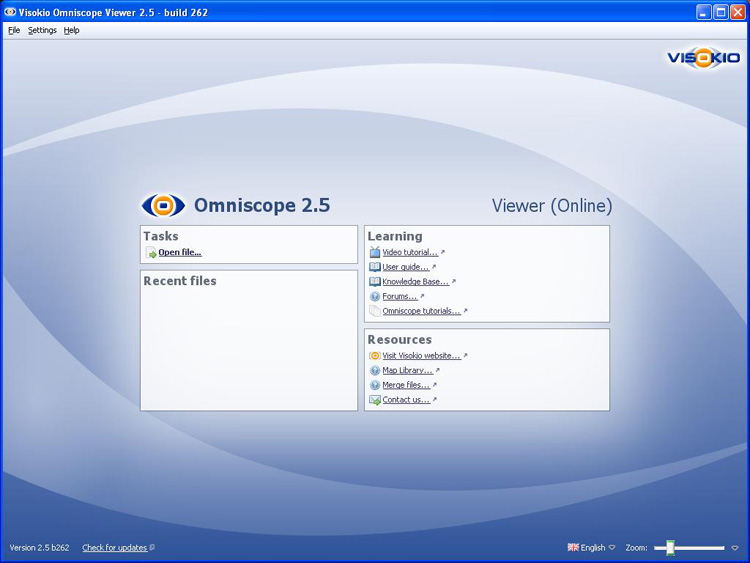
{update to version 2.5 in progress}
Omniscope offers options to print from individual views, or at the level of the entire file. In addition to printing only one view, or the current page, it is also possible to print some or all tabs as PowerPoint or Adobe Acrobat files, with many options to show or hide various aspects of the Omniscope display in the printed versions.
Sometimes, you may wish to print a single view on a single piece of paper. All views offer this option from View Tools > Capture Views > Print. Right clicking on views with backgrounds, like the Pie and Graph Views, also presents a view Print option.
If you are running Windows, the individual view print option available from Capture Views > Print will launch the Windows Page Setup dialog enabling you to confirm the paper size, orientation and margins for the page you wish to print.
 | 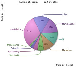 |
Note: When printing individual views, the view title does not print.
Sometimes, you would like to print a paper copy of the entire page display, or multiple tabs, from Omniscope. On the Main Toolbar, File > Print opens a printing options dialog:
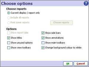
Choose reports:
Current display/report only - prints only the current tab displayed in Omniscope
Include all reports - prints all the tabs in the file.
Print some reports - allows you to choose which tabs you wish to print from a drop-down pick list
Display options:
Show report tabs - unless ticked, Report Page tabs are not printed
Show side bars - when ticked, Side Bars are printed on each page.
Show titles - when ticked, the page titles are printed (view titles are always printed when printing pages)
Show annotations - when ticked, prints the annotations below the views on each page
Show unused options - unless ticked, does not print aspects of the display relating to unused options, e.g. Pane-by menus are not displayed in views with no active paning.
Show Main Toolbar - unless ticked, the Main Toolbar does not print
Show view toolbars - unless ticked, the View Toolbars do not print
Change background colour to white - when ticked, substitutes a white background when printing
File > Print as PowerPoint launches the Print Options dialog described above. You can choose to print the current display, or some or all the Report Pages configured in your file. Click on OK and Omniscope processes the pages you have selected. When it finishes, Omniscope displays the Print as PowerPoint wizard:
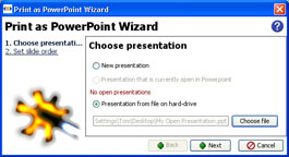 |  |
If you want to create a new PowerPoint file, choose New presentation. If you already have your PowerPoint file open, choose it from the list of open presentations. Otherwise, browse to and open the PowerPoint file you wish to add pages to. If you are adding pages to an existing PowerPoint file, you are asked where to insert them:
Warning: If you specify Replace existing slide, make sure that the slide number choosen is a blank 'placeholder' slide or otherwise uneeded; it will be overwritten and all addtional pages inserted behind it. Subsequent slides will not be overwritten.
Click on finish and Omniscope will open the PowerPoint file. If you wish to save or print this file, you can now do so from PowerPoint itself:
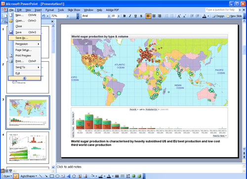
File > Print as PDF launches the Print Options dialog described above. You can choose to print the current display, or some or all the Report Pages configured in your file. Click on OK and Omniscope precesses the pages you have selected. When it finishes, Omniscope displays the Print as PDF wizard:
Specify the new file name and location you want to save this file. Open the file to access the full range of options for managing .PDF files, including printing.
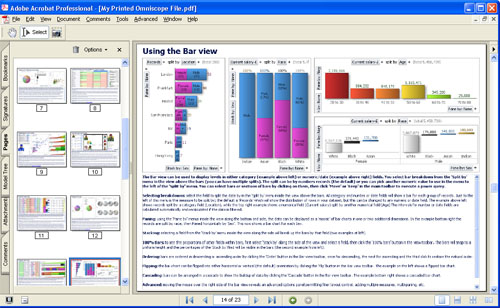
Applies to versions 2.3 & 2.4
This section provides an introduction to 'navigating' or 'exploring' Omniscope files that someone else has prepared and sent to you. This section uses an Everton British football club file as an example, which you should download now [480].
Omniscope files always open as last configured and saved. In the case of the Everton file, it has many columns that could be used for filters, so it has been configured to open with four views and both the right and left Sidebars open:
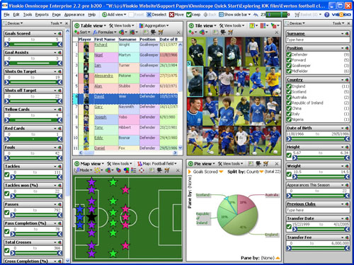
The following sections discuss the navigational features on the Omniscope Main Toolbar, and the use of Sidebar filters and other devices that help you navigate any IOK file and select the records (rows) that you wish to see in detail.
![]()
The left side of the Main Toolbar contains top level command menus useful for preparing .IOK files. These are not needed to navigate .IOK files already prepared by someone else with your needs in mind. More detail on these commands, which are not specific to using individual views, can be found here [481]
To the right of the command menus, the Main Toolbar displays a number of useful icons/buttons that are used to aid exploration/navigation of the .IOK file:![]() Add View - Used to add an additional View to the current display. In the demo, try adding a Details View to the display. To remove a View from the display, click on the [X] in the upper right hand corner. To change one View to another, click on the View name and select the View you want from the drop-down menu. In the demo, try changing the Map View to a Graph View.
Add View - Used to add an additional View to the current display. In the demo, try adding a Details View to the display. To remove a View from the display, click on the [X] in the upper right hand corner. To change one View to another, click on the View name and select the View you want from the drop-down menu. In the demo, try changing the Map View to a Graph View.![]() Reset - Omniscope files are flat tables of data, with records (rows) and fields (columns). One of the objectives of navigating an Omniscope file is to select and focus on only a certain subset of records (rows), rather that the whole universe of records in the file. The Reset button removes all of the filtering criteria you may have expressed, and returns the current display views to show all the records. It is very important to always reset your data before filtering, so that all qualifying records will be considered in your subsequent query.
Reset - Omniscope files are flat tables of data, with records (rows) and fields (columns). One of the objectives of navigating an Omniscope file is to select and focus on only a certain subset of records (rows), rather that the whole universe of records in the file. The Reset button removes all of the filtering criteria you may have expressed, and returns the current display views to show all the records. It is very important to always reset your data before filtering, so that all qualifying records will be considered in your subsequent query.![]() Deselect - Omniscope navigation depends on 4 basic operations: Select (or Deselect), Move, Keep, and Reset. Every view provides ways of selecting one or more records. In the Everton demo file, look at the Table View and under 'Player', click on the first picture (Richard Wright). His record is now selected, indicated by blue animated shading, and his record is now highlighted in other views. In the Graph View, for example, we can see from the blinking highlight that like most goalkeepers, he had no goals or assists. Now click the Deselect icon on the main Toolbar, and this record is not longer selected. Try selecting, then de-selecting other players, or groups of players. For example, in the demo Pie View, click on Republic of Ireland. This will select two goal-scoring players from Ireland. Be sure to click Deselect before moving on.
Deselect - Omniscope navigation depends on 4 basic operations: Select (or Deselect), Move, Keep, and Reset. Every view provides ways of selecting one or more records. In the Everton demo file, look at the Table View and under 'Player', click on the first picture (Richard Wright). His record is now selected, indicated by blue animated shading, and his record is now highlighted in other views. In the Graph View, for example, we can see from the blinking highlight that like most goalkeepers, he had no goals or assists. Now click the Deselect icon on the main Toolbar, and this record is not longer selected. Try selecting, then de-selecting other players, or groups of players. For example, in the demo Pie View, click on Republic of Ireland. This will select two goal-scoring players from Ireland. Be sure to click Deselect before moving on.![]() Move - Selecting records is a precursor to deciding whether to Move these records OUT of further consideration. The Move Command moves all selected records OUT of consideration, where they stay until the display is Reset.
Move - Selecting records is a precursor to deciding whether to Move these records OUT of further consideration. The Move Command moves all selected records OUT of consideration, where they stay until the display is Reset.![]() Keep - the opposite of Move, the Keep command keeps only the selected records IN consideration, and moves all the other unselected records OUT of consideration.
Keep - the opposite of Move, the Keep command keeps only the selected records IN consideration, and moves all the other unselected records OUT of consideration.![]() Back - like a browser, you can go back to the previous display at any time by pressing Back.
Back - like a browser, you can go back to the previous display at any time by pressing Back.![]() Controls (2.3 Show Sidebar) - clicking this icon gives you the option to show or hide the Sidebars on one or both sides of the current display. Uses of the Sidebar are explained in the section on filtering.
Controls (2.3 Show Sidebar) - clicking this icon gives you the option to show or hide the Sidebars on one or both sides of the current display. Uses of the Sidebar are explained in the section on filtering.![]() Barometer - upon opening a file, it is useful to know how many records are in the data set. As you filter, it is useful to see how many records have been kept IN consideration, and how many moved OUT. The barometer is a visual gauge that shows the total, as well as the split between IN (green) and OUT (red). Click on the Republic of Ireland wedge of the Pie View in the demo. Notice how the barometer tells you that you have selected two players.
Barometer - upon opening a file, it is useful to know how many records are in the data set. As you filter, it is useful to see how many records have been kept IN consideration, and how many moved OUT. The barometer is a visual gauge that shows the total, as well as the split between IN (green) and OUT (red). Click on the Republic of Ireland wedge of the Pie View in the demo. Notice how the barometer tells you that you have selected two players.
Now click ![]() Move. Notice how the barometer tells you that you have excluded two players...just because they were Irish?
Move. Notice how the barometer tells you that you have excluded two players...just because they were Irish?
Since they were goal scorers, let's click ![]() Reset and put them back on the team!
Reset and put them back on the team!![]() {version 2.3 only} Basket - the basket is a 'parking place' where you can put selected records, such that they will stay there even if you Reset the display. At any time, you can open the Basket and see the records you have placed there. In the demo, go to the Table View and select the Position 'Goalkeeper' instead of Richard or Wright. Notice that unlike a spreadsheet, the Barometer tells you that you have selected 3 Goalkeepers, not just Richard Wright. Now click the Basket, and choose 'Add selection to basket'. The record count in the Basket changes to 3. To view the contents of the Basket, click on the icon. We have just put all 3 of our Goalkeepers on the market! Let's re-consider...click on the drop-down arrow to the right of the basket, then click Clear selection from basket, or Clear basket. More on Using the Basket [482].
{version 2.3 only} Basket - the basket is a 'parking place' where you can put selected records, such that they will stay there even if you Reset the display. At any time, you can open the Basket and see the records you have placed there. In the demo, go to the Table View and select the Position 'Goalkeeper' instead of Richard or Wright. Notice that unlike a spreadsheet, the Barometer tells you that you have selected 3 Goalkeepers, not just Richard Wright. Now click the Basket, and choose 'Add selection to basket'. The record count in the Basket changes to 3. To view the contents of the Basket, click on the icon. We have just put all 3 of our Goalkeepers on the market! Let's re-consider...click on the drop-down arrow to the right of the basket, then click Clear selection from basket, or Clear basket. More on Using the Basket [482].![]() Help screen - click on the help icon to see what the publisher or re-publisher of the file may have to say that will help you understand more about the file.
Help screen - click on the help icon to see what the publisher or re-publisher of the file may have to say that will help you understand more about the file.![]() Publisher logo link - if you are publishing or re-publishing a file, you can put your own logo here, and link it to your website.
Publisher logo link - if you are publishing or re-publishing a file, you can put your own logo here, and link it to your website.
Most Omniscope files contain pages with Sidebars showing on the right, the left or on both sides of the display. At any time, you can reveal and configure Sidebars to help you and your readers navigate a file.
{version 2.4 only} The display of Side Bars is controlled from the Main Toolbar > Controls drop down menu. More infomation on configuring and using Sidebars [483] and using the Controls [484] drop-down.
| In the Sidebar text device labelled 'Surname', type a letter. Notice how all views update to display only players whose surnames begin with that letter. Back-space or click Right-clicking on a Sidebar device reveals a wealth of options to change things, such as resetting all the other filters or even hiding the filter. To return all Sidebar filter settings to their original state, click the global |
Unlike free Viewers, an activated Omniscope can import data from any number of different sources, and can combine disparate, even unrelated tabular data sources into a single, in-memory Omniscope file. Current versions of Omniscope assemble data into one 'flat' tabular, in-memory structure (called a data set although any number of unrelated tabular data sets can be appended into one file). All source file locations, database connections, merges and appends and other transformations required to assemble and refresh a given data set are remembered and re-executed by Omniscope on file open or on refresh.
DataManager (2.6+) [398] The DataManager workspace usually appears on its own tab and provides a highly-visual drag-and-drop interface for defining and importing data from various sources. The same workspace can also be used to define how data is assembled and transformed prior to loading into Omniscope's in-memory structure, and how many output files and distribution delivery options are defined for a give Report IOK file. Many (but not all) of the options available via the DataManager workspace are also accessible from the Main Toolbar File: and Data: command menus. Operations defined in these menus are also visible by opening a DataManager tab from Tab > New > DataManager. A DataManager View workspace can be combined with other views by adding them to the DataManager Tab. By default, a Table View appears below the DataManager workspace, although it will not be populated until you select a data block to Load.
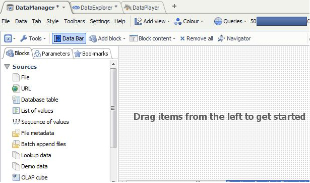
More on importing data using the DataManager Sources menu [398]
The same import blocks as are accessed via the Datamanager workspace can also be accessed from the Main Toolbar: File > menu
Open a new file and you will see a blank table similar to a spreadsheet where you can type or cut-paste data or text into cells. Populating your own small, experimental IOK file by typing in sample data is an excellent way to get started with Omniscope. You can also cut-paste tabular data sets from documents or web pages to provide a starting point. From the Main Toolbar File menu or Welcome Screen, select File > New [399] and specify how many blank rows and columns you will start with.
Omniscope can automatically open supported [473] delimited data files and import a copy of the tabular data, either locally, across the network or over the web using a URL. Using the DataManager tab workspace, drag a File Connector block from the Sources menu onto the workspace for each file you wish to import
Using either vendor-specific or generic ODBC or JDBC protocols, Omniscope can establish and refresh direct connections to relational database tables and reporting views. From the DataManager tab workspace, drag a Database Connector block onto the workspace and configure it for each table/reporting view you wish to import into the file.
See the KnowledgeBase [474] section on database connectivity for worked examples and more technical detail on advanced database integration options, e.g. parameter-passing to enable variable 'on-demand' data imports using parameter passing and parametric SQL statements to automatically vary the size/granularity of the data sets being imported.
The new Database Connector blocks replace the Database Connection Wizard (2.5) [485]
OLAP cube connections [486]
Opening folders of files [487]
Batch append files [488]
Open online source/feed [489]
See Using Connectors [403] for more detail on how to use specific Connectors
Open a map [401] - download a map, and add data to the file, including positioning record markers on the map
Beginning with version 2.6, Omniscope features a new drag-and-drop visual workspace enabling non-technical users to import, assemble, transform (aggregate, de-pivot, tokenise, etc.), filter, sample, scramble and export tabular data sets, with no knowledge of SQL.
File [490] | List of values [491] | Batch append files [492] | OLAP cubes [493] | Operations [494] |
| URL [495] | Sequence of values [496] | Lookup data [497] | Online Sources/Connectors [498] | Outputs [499] |
Database table (or view) [500] | File metadata [501] | Demo data [502] | Merging feeds [503] |
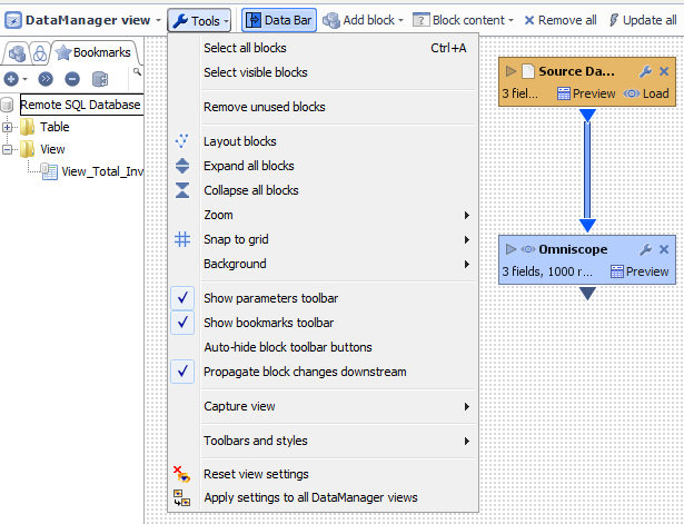 | View Toolbar |
Block Tools: Block note: allows the user to insertcomment in the Block Rename: allows the user to Remane theBlock name Load into Omniscope : Load datainto Omniscope Update data: Load data from Omniscope(Table)to the block. Update Option: These settings allow you to customise howOmniscope checks for changes for this block. =>can be Never-Auto or Scheduled Preserve formulas output:Keep the formula when creating an output file. Create duplicate : does createa duplicate of the block Create a snapshot: Create asnapshot of the block Replace with snapshot: Replacethe block with a snapshot. Bookmark This block: will create a“shortcut” under Bookmark menu Explore to: Allow you to open a file Reset size: reduce the size of the block Maximize: Maximize the size of the window Remove others: Remove ALL of the blocks except for 'Rename(snapshot)'? Remove: Remove the block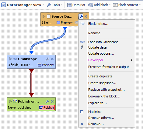
Sources - using DataManager source blocks
Omniscope DataManager workspace opens to reveal a Data Bar/Blocks menu on the left side, and an Add Block menu is always available at the top of the drag-and-drop workspace.
The user can importe an Excel file including X number of worksheets, Omniscope will give the user the possibility to choose, individual, or a pair of working sheets:
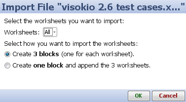 | -The name of the worksheet will appears under the buttonAll.
-The user can also create one block and append X number of Worksheet. or create one block for each worksheet |
By clicking on the block the user is able to:
-See/change the directory of the file.
-Change and modifythe setting of the Table Data
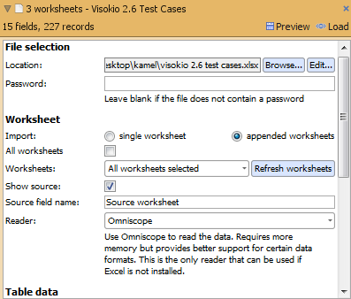 | 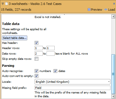 |
Data Manager also gives the possibility to change thesetting of the table if the user use the option selects table data.
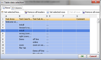 | This Option gives the possibility to Configure/Select or Remove any rows, column and Headers. |
URL
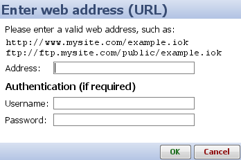 | Data Manager can Import data from a remote data file such as an XML, CSV file or a SpreadSheet. |
To see how to configure the Database in DataManager click Here [402]
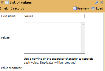 | List of values Block create a list of values that you can use as input to create any operation. |
Sequence of values
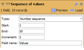 | Sequence of values generate a sequence of values betweenStart and End values. |
File metadata
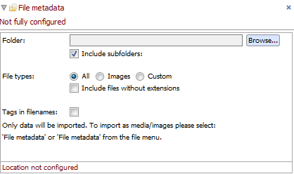 | FileMedia data Block, retrieves all information about all of the media files in afolder. |
Batch append files
location of data files to be automatically appended into a single data set.
 | Batch append files, appends a set of files whith in a designated folder |
Lookup data
useful data available for free
 | Look up, Imports data from one of the Omniscope sample files to DM |
Demo data
 | Same as Look up option, Demo data Imports data from one of the Omniscopesample files |
OLAP cubes [486]
The OLAP cube source block provides connectivity to MDX-compliant multi-dimensional data structures (cubes) such as Microsoft SSAS and other cubes.
 | OLAP cube, Import data from an OLAP Cube such as SQL Server Analysis Services. |
Online Sources/Connectors [403]
 | Under the Blocks > Sources menu, the DataManager workspace provides access to a growing number of Online Sources/Connectors allowing you to control the import of data from remote sources to which you have access. Connectors enable Omniscope to access structured data sources unique to a publisher/platfrom or application directly via API calls, rather than via exported delimited data files or views/tables from relational databases imported using SQL statements and JDBC/ODBC protocols.
Note: Connectors for accessing, refreshing and synchronising with remote-hosted 'clouds' are available only from activated Omniscopes, not the free Viewer. |
Other Data Bar Blocks in DataManager:
 | Online data sources ranging from freely-available searchable sources like Twitter and web searches to premium real-time data feed services like Bloomberg. Using Merging feeds [504] |
Operations
 | The DataManager workspace also allows you to define any sequence of transformational operations by dragging Operations blocks onto the workspace. Operations blocks are also accessible from the Mani Toolbar Data > Operations menu and are fully documented here. Transforming Data [505] |
Outputs
 | Any number of different file output, publishing and distribution options can alo be defined using the DataManager data flow definition workspace. Output/export and disctribution/devliery options are fully documented here. Defining Outputs [506] |
Under the Blocks > Sources menu, the DataManager workspace provides access to a growing number of Online Sources/Connectors allowing you to control the import of data from remote sources to which you have access.
Connectors enable Omniscope to access structured data sources unique to a publisher/platfrom or application directly, rather than via exported delimited data files or views/tables from relational databases imported using SQL statements and JDBC/ODBC protocols.
Note: Connectors for accessing, refreshing and synchronising with remote-hosted 'clouds' are available only from activated Omniscopes, not the free Viewer.
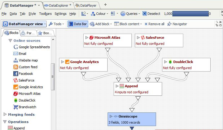
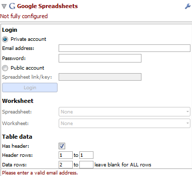 | The user is able toimports a worksheet Spread Sheets created on Google Spread sheet into DataManager: http://www.google.com/google-d-s/spreadsheets/ [507]
DataManager gives also the possibility to load and View a public spreadsheet by copy and past a Link/key. Google spreadsheets are on-linecollaborative tools for Gathering and maintaining structureddata sets.
How to use Omniscope with Google Spreadsheets [406]
|
Email Connector
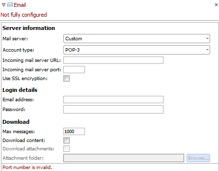 |
The user is able to imports email data from a POP3 or IMAP email account.
A list of server will appearwhen click on Mail Server option box, the user is able to select any Serverused. The user is able to setupthe Max number of messages he wants to seen in Omniscope. DataManager gives also thepossibility to load the Messages content and any attachements. How to use the
|
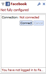 | Datamanger allows the userto import data from FaceBook. Facebook [508] is a social networking applicationthat allows users to create networks of relationships centred on theiraccounts. How to use |
Google Analytics
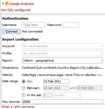 | The user can import report, data from Google Analitic, and also provideswebsite traffic and marketing information: http://www.google.com/analytics/ [509]
DataMager allow the user to filter the data by time/Visitor/content.
The Google Analytics import functionallows you to download and analyse Google Analytics data from within Omniscope. How to use
|
Web Mapping
A web site map is a network of interconnecting pages within a particular website. A connection between two pages exists if the first page contains a link to the second page. You can use the webmap functionality within Omniscope to visualise the structure of a website.
How to use Omniscope for Web Site Mapping [409]Salesforce [510] is an application that runs in the Force.com [511] online cloud-computing hosted platform, one of the largest and fastest-growing general-purpose SaaS platforms. Salesforce is widely used for CRM (Customer Relationship Management, composed of the 'Sales Cloud' and service/case management, aso know as the 'Service Cloud'). Almost any application can be written on the Force.com platform. If you have a Salesforce account, it is possible to access your Reports and Data Objects/Tables stored in Salesforce using either the Omniscope direct connector (File > Open online source > Salesforce) or the free web connector [512] your Administrator can install into your Salesforce account from the online AppExchange [513].
Salesforce web connector: the free Omniscope Connector for Salesforce [512] web service can be installed in your Salesforce account(s) from the AppExchange listing page [512] by your Administrator, unless you have a Group Edition. Instructions for installing in Group Editions are here. The web connector installation will add a new tab from which you can download reports and un-joined data objects using pre-configured templates to deliver files that will open in the free Viewer. An activated version of Omniscope is required to modify and save customised templates, which can then be uploaded to your account, adding new download and viewing options for different classes of users within your organisation. More on using the online Web Connector for Salesforce [514].
Salesforce direct connector: Omniscope Professional and Enterprise 2.5 (and later) enable to access your Salesforce reports and data objects directly. More on using the Direct Connector for Salesforce [515]to access, modify, edit and synchronise changes with your Salesforce-hosted data.
More detail and a solutions roadmap for making the most of the combination of Salesforce and Omniscope is here [410].
(experimental feature)
(experimental feature)
If you would like to discuss developing an Omniscope Connector for your remote data ASP/SaaS platform, client-premise installed application, or online data service, please contact us. [86]
Omniscope version 2.5 and beyond include a connector that can import e-mail from any online email account supporting either the IMAP or POP-3 email management protocols. Most modern web-based email accounts support at least one of these protocols.
To import email data into Omniscope, select File > Open online source > Email. The Account details dialog will be displayed:
| Mail server - Select your email server. If your email server does not appear in this list you should select the 'Custom' option. Accounttype -This option is only enabled if you select the 'Custom' mailserver. Select the type of email account (either POP-3 or IMAP). Incomingmail server URL - This option is only enabled if you select the 'Custom'mail server. Select the address of the mail server. Incoming mail server port - This option is only enabled if you select the 'Custom' mail server. Enter the mail server port. UseSSL Encryption - This option is only enabled if you select the 'Custom'mail server. Check this box if your email server uses Secure SocketsLayer encryption. Username - Enter the username you use to log-in to your email account. Password - Enter the password you use to log-in to your email account. Maxmessages - Determines the maximum number of email messages that will bedownloaded. A value of '10' means the 10 most recent messages will bedownloaded. Download content - Check this box if you want todownload the message content. This will enable you to read messageswithin Omniscope but will also increase the size and amount of datadownloaded. Download attachments - Check this box if you want todownload message attachments. If this option is selected, then you mustalso specify a valid attachment directory. Attachment directory - This determines the folder attachments are moved to after they have been downloaded. |
Once you have entered the relevant information click the 'OK' button to start downloading the message data. A status dialog will be displayed to show you how many messages have been downloaded and how many are still to come:
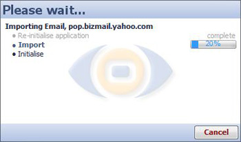
Google Docs and Spreadsheets [516]is a free service that enables anyone to create documents, spreadsheets and presentations online. You can import and collaboratively edit or publish from .doc, .xls, .csv, .ppt, .txt, .html, .pdf and other formats. You can export files for use with traditional desktop software as well.
Hosted online spreadsheets enable powerful new workflows with collaborative data compilation and editing options...no more playing 'file tag' with offline spreadsheet files circulating as e-mail attachments. These so-called 'cloud' solutions enable co-workers to share the same online copy of each document, spreadsheet or presentation. All revisions are saved and recoverable.
Omniscope will connect to any Google spreadsheet and edit it online in the browser or off-line in Omniscope. Changes will be synchronised between Omniscope and Google Spreadsheets in real time. The combination permits collaborative compilation and maintenance of data sets delivered in branded, highly-visual Omniscope files with the possibility of live refresh and banner ads inside the file.
Combining Google's free hosted online spreadsheets with Omniscope provides a 'best of both worlds' solution enabling many new workflow and publishing options. Data publishers and most businesses can benefit greatly by shifting most typical spreadsheet data compilation and maintenance workflows to an online spreadsheet linked to Omniscope.
When you create a new Google Spreadsheet, there are two ways of inviting others to help compile, edit and maintain the data. For data being published to the public, you can define a link or key allowing anyone with the link to connect to the data using Omniscope, and optionally help to edit the data. Once this link is embedded in the Omniscope file, this source worksheet will be remembered and data refreshable in activated Omniscopes from the Omniscope file. For company internal data, you can use the more Google Docs Share with others dialog to determine who will have what type of access to the spreadsheet, who can make changes etc.
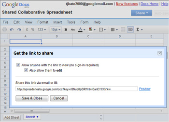 | 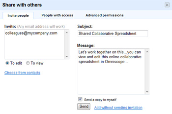 |
To create an Omniscope file from a Google Spreadsheets worksheet (either private or public) as a linked data source, go to File > Open online source > Google Spreadsheets. Enter your account details for private spreadsheets, or the link or spreadsheet key to use public spreadsheets. Once you have logged into your account or connected to a public spreadsheet, select the worksheet that will be the linked data source for this Omniscope file.
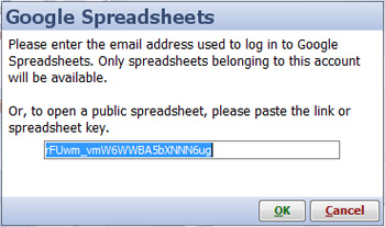 | 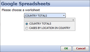 |
Omniscope will automatically import the data and open in the default layout. You can further configure the layout of the Omniscope file, then save it as an .IOK/.IOM file. The default refresh behaviour with online data sources is 'Never', since you may want to open the file while offline. If you or your colleagues have activated Omniscopes, while online you can use Data > Refresh from source for on-demand refresh, or you can go Data > Automatic Refresh to configure automated refresh based on frequency of polling timings you can configure. If you plan to always open the file while online, you may choose to save it with refresh set to 'Always'.
You can save an Omniscope file whose linked data source is a Google spreadsheet with the refresh behaviour set to 'Always', and the file will update itself with the latest data from the Google spreadsheet. You can also activate and configure Automatic refresh to keep the Omniscope file updated while open.
You can view the linked data source spreadsheet from the Omniscope file using the Web View. Files using the Google Spreadsheets connector open by default to display the linked spreadsheet in a Web View:
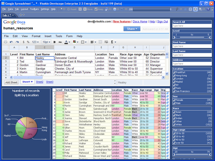
Google Analytics is a free online service that allows you to monitor various statistics about visitors to your website(s). In order to use Google Analytics you will need to sign-up and then configure your web-pages to generate the required information. Once you have signed up you can log-in to the Google Analytics website to view and analyse your website analytics data. To sign up for Google Analytics or to get more information click here [509].
Omniscope allows you to download Google Analytics data straight to your desktop. This means you can use Omniscope's powerful visualisation environment to quickly and effectively download and analyse all of the data for any Google Analytics report in one go.
To import Google Analytics data select File > Open online source > Google Analytics. A dialog will be displayed asking you to enter your Google Analytics username and password. Enter the same username and password that you use to log-in to the Google Analytics website.
|
Once you have entered your username and password click the 'OK' button. Omniscope will attempt to contact the Google Analytics server. If the server was contacted successfully and your username and password are valid the report configuration dialog will be shown. This dialog allows you to specify what Google Analytics data you want to download.
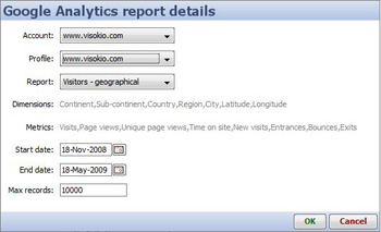 | Account - Select your Google Analytics account. Profile - Select your website profile. Report - Select from one of 8 pre-defined Reports or choose 'Custom' to generate a custom Report. With Custom Reports you can specify the information you want to download and how you want it to be organised. To configure a Report, select a combination of dimensions and metrics. Dimensions determine how the data is segmented, such as browser type, visitor city or language. Metrics provide data for the selected dimensions, such as the number of visitors, unique page views and bounce rate. Start date - Select the start date of your data. End date - Select the end date of your data. Max records - Define the maximum number of records you want to download at once. |
When you are happy with the configuration click the 'OK' button to download the data from the Google Analytics server into Omniscope.
New in 2.5... this page in progress
In Omniscope 2.5 and beyond you have the ability to generate a website map and view the site and associated data on content and structure in Omniscope.
To generate a website map you need to provide Omniscope with one or more 'seed' URL's. Omniscope will 'crawl' and then download the contents of each of these URLs and extract all the links. The content of each of the linked pages is then downloaded and the content extraction process is repeated. The resulting data set contains the details of all of the pages downloaded and the connections that exist between these pages. This can be visualised in Omniscope using the Network View to show a 'map' of all the pages, with each node in the map representing a page and each line representing a link between from one page to another.
A website map can prove useful in many different scenarios:
To generate a web site map select File > Open online source > Website map.
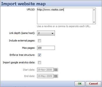 | URL(s) - Enter one or more URL's to use as a starting point for the website map. Include external pages - most web sites include links to pages on other sites. When ticked, this option includes pages from other sites referenced by links.
|
Import Google Analytics data - when checkedOmniscope will attempt to retrieve Google Analytics information for anyof the pages encountered that belong to one of the sites associatedwith a Google Analytics account to which you have access. If you select this option then youwill have to enter a Google Analytics username and password. Moreinformation on the Google Analytics functionality within Omniscope canbe found here [408].
Start date - only available if the 'Import Google Analytics data' option is checked. Select the start date for the Google Analytics data.
End date - only available if the 'Import Google Analytics data' option is checked. Select the end date for the Google Analytics data.
 | 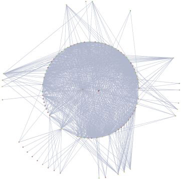 | |
Enforce tree structure selected | Enforce tree structure unselected |
Using Omniscope with SalesforceAdd the perfect desktop/web compliment to Salesforce solutions |
Omniscope is integrated with Salesforce and the Force.com [517] cloud computing platform and provides a low-cost, low-risk route to business intelligence reporting and data quality initiatives involving data hosted in Salesforce/Force.com. If you have a Salesforce account and security token, you can go to File > Open online source and choose to open either a Report (read-only) or Data Object/Table directly from Salesforce. Using the direct connector, you can you can visualise, analyse, save offline, add/edit data and synchronise your changes with Salesforce. There is also a free web connector for Salesforce listed on the AppExchange [512].Your Administrator can install a 'Visokio Reports' tab into your Salesforce accounts to enable pre-configured downloads of Reports and Data Objects/Tables that open in the free Viewer. Using an activated Omniscope, you can also modify the default templates provided for each Report and Data Object/Table, and upload your customised files to the'Visokio Reports' tab in Salesforce to modify the online DataPlayer displayed or provide alternative templates for future downloads. The free web connector can be installed in Group accounts, but the direct connector involves API access which Salesforce permits only to subscribers with Professional, Enterprise and Unlimited Editions.
Start by installing the free Omniscope Connector for Salesforce 2.1 [512] (a certified, AppExchange-listed application) into your Salesforce user accounts. Salesforce Administrators can do this automatically from the AppExchange if your organisation has the Professional, Enterprise or the Unlimited editions of Salesforce. If your organisation uses Salesforce Group Edition, any Administrator can install the Connector tab manually by following these directions. [518]
Installing the web connector will add a new 'Visokio Reports' tab to some or all of your user accounts. From this tab, users with the free Omniscope Viewer [519] installed can download, view, filter and query the data in their Reports. The look and feel of the files will initially be based on the standardised default Omniscope file templates provided for each Report or Data Object. During your free trial, you can modify these template files and upload them for others to use when downloading to the free Viewer. Users without the free Omniscope Viewer installed cannot open local copies of their data from the permissioned tab, but can still use interactive Flash DataPlayer 'dashboards' you can create and export from Omniscope to your Visokio Reports web tab. For more details, see using the web connector. [514]
If you install Omniscope [450], and you have Professional, Enterprise or Unlimited editions of Salesforce, during your free trial you can not only modify templates and save/archive secured copies, you can also access Reports and Data Objects directly using the File > Open online source > Salesforce login and download option (you will need to paste-in your security token). Using Omniscope Professional or Enterprise, you can connect to and edit Data Objects offline, then synchronise your changes with Salesforce using the Data > Synchronise with Salesforce wizard. For more details, see accessing Salesforce directly from Omniscope [515].
Once your 30-day free trial period has expired, upgrading your Omniscope from free Viewer to the Professional or Enterprise Edition enables you to continue modifying and uploading customised templates and DataPlayer 'dashboards', integrating/merging in data from non-Salesforce sources, saving and sharing secured Omniscope files offline, and synchronising offline changes back to Salesforce. Non-activated Omniscope installations will revert to being free Viewers able to download and filter/query default or customised files from the free web connector tab installed in the user accounts. No need to uninstall.
For the quickest start, maximum flexibility and lowest average cost-per-user in deploying your solution, use the Salesforce:
Installing the free Omniscope Viewer/Professional trial and the free Visokio Reports web tab from the AppExchange enables any organisation to embark on a simple, low-cost, low-risk, ‘tiny-steps' progression of continuous improvements, while delivering users live, working reports with many useful visualisations of their data beginning on Day One:
1. Install free Omniscope Viewers and add the free Visokio Reports web tab to user accounts
a. Download key reports/data objects from each user's account tab using the standard templates, enabling users to see, filter and sort all their data to find alert conditions, data errors & inconsistencies.
b. Ask users to start flagging incomplete, out-dated and erroneous data records/fields online in Salesforce using the unusual "!" character or similar
c. Download key data objects as Omniscope files and consult the Flagged Errors tab to view all the records which have been flagged for online correction/completion either online via Salesforce, or offline using an activated Omniscope Professional and the direct connector for Salesforce, available in the free 30-day trial.
d. Create custom reports containing the most useful joins...users can then download and view standard template versions of these reports using Omniscope.
e. File refresh & security - the data in Omniscope files downloaded in templates is always fresh, and cannot be exported or copied (not even cut-and-paste). Users of free Viewers cannot save the files...they must always return to their Salesforce account Visokio Reports tab to download fresh copies of the data or view online DataPlayers in sub-tabs.
2. Upgrade to Omniscope Professional (requires activation)
a. If your 30-day free trial has expired, contact us [86] to purchase a licensed activation key to upgrade from free Viewer to Omniscope Professional.
b. Now you can continue to modify and save files downloaded from your Salesforce account tab to fit the needs of your organisation - adding/changing report tabs to highlight key messages, introducing corporate branding, etc. Make multiple versions of each report/data object template to suit the needs of different classes of users.
c. Save your changed .IOK file(s), then upload one or more of your modified files from the Visokio Reports tab in your Salesforce account. Note: you can upload the file empty, with all data deleted... data in the uploaded template file(s) will not be synchronised with the online data.
d. Modify the standard Flash DataPlayers shown in the DataPlayer View tab of each template file downloaded, then export your new customised DataPlayer ‘dashboard' to web pages (including Salesforce tabs) and/or internal documents such as PowerPoint, Excel or .PDF.
e. The custom templates/DataPlayer configurations uploaded will be selectable for future downloads from the Visokio Reports tabs of authorised users, whether using the free Viewer or a Professional.
f. Data integration projects: download custom versions of your reports/data objects and then use Omniscope to merge in related data from other sources (spreadsheets, ERP databases, etc.) to create combined reports (using any number of joins)that can be circulated to users with the free Viewer.
g. Using Omniscope 2.5 or later, you can also login to your Salesforce account from inside Omniscope, connecting directly to reports or data objects using File > Open Online Source > Salesforce Table/Report
h. Use the powerful data cleansing/scrubbing and editing capabilities of Omniscope to make changes to your data and save local copies of files.
i. Using Omniscope 2.5 or later, use the Data > Synchronise with Salesforce command to make changes to both your local copies and the corresponding user-editable fields within your Salesforce organisation.
j. File refresh & security- Users with Professional Editions will be able to refresh directly from source on opening. Offline files sent to users with the free Viewer show configurable opening screen ensuring they do not use stale files.
k. Continue to optimise the configuration of templates for all your reports and data objects based on user feedback and the evolving needs of your business...enjoy the total flexibility of the hybrid solution you have created.
3. Automate refresh, archiving copies and distribution with Omniscope Enterprise Edition
a. Omniscope Enterprise edition is designed to automate the entire process of refreshing and distributing Omniscope reports and Flash DataPlayer inserts from a central 'always-on' server with access to all the required data sources, including Salesforce.
b. A single Enterprise Edition allows automated refreshes of files with data from Salesforce and other sources, plus distribution (via e-mail or FTP) of refreshed IOK files and DataPlayer dashboards either according to a defined schedule or on-demand using the Scheduler or the Generator, two automation tools included with Enterprise Editions.
c. File refresh & security - Enterprise installations offer the full range of file security options, including time-limiting and domain-locking of files (files will not open if user is not logged into specified site and download page e.g. Salesforce)
Using the Salesforce Visokio Reports TabInstall this free service in any Salesforce Edition, including Group Edition |
The Omniscope web connector for Salesforce is a certified, AppExchange-listed free service [512] that can be installed by your Salesforce Administrator in any Edition of Salesforce, including Group Edition. Once installed, the new web connector tab provides your users with one-click downloads of pre-formatted, filterable, highly-visual, offline copies of Salesforce Reports and Data Objects/Tables. The downloaded files can be shared as presentations with anyone using the Omniscope free Viewer. Each file download contains all the data [454], configured as multi-tabbed visualisations and report.
|
If you are running the Professional, Enterprise or Unlimited Edition of Salesforce, and you are logged into an Administrator account, you can install the free web connector service just by clicking the [Get It Now] [512]button. If you are running Group Edition of Salesforce, you can still install the web connector manually following these instructions [521]. Once installed, the web connector tab appears at the right-most end of your opening tabs, usually with the label 'Visokio Reports'. Click on the tab At the top of the tab is a link for all users to install a free Omniscope 2.5 [519] Viewer, with free 30-day trial of Omniscope Professional authoring capabilities anyone can use to modify the default templates. | |
| Select Report or Data Object/Table to download * not available when installed in Group Edition | |
| Your data will open in your installed Omniscope | |
| If you like, customise templates and upload Use Omniscope Professional to customise template files for different purposes or user groups. All template .IOK files can be downloaded and interacted with using the free Viewer, dramatically reducing average cost-per-seat of your Business Intelligence and reporting solution for Salesforce. |
WARNING: due to limitations imposed by Salesforce, when installed in Group Edition accounts, the Omniscope web connector does not support upload of customised templates, and displays All Reports, rather than the custom "My Reports" tab by default.
Group Edition installs are not done using the [Get it Now] button on the AppExchange. they must be done manually following these instructions:
To begin, go to www.salesforce.com [510] and make sure to login to an account with a System Administrator profile
Click "Setup" at top of screen
In left side panel under "App Setup" click "Create" to expand menu
In expanded section under "Create" click "Tabs"
In the middle "Web Tabs" (not "Custom Object Tabs" above or "VisualForce Tabs" below) box, inside the Web Tabs header, click the grey "New" button centre
Step 1. Choose Tab Layout, choose "2 columns with Salesforce sidebar"
Click "Next"
Step 2. Define Content and display properties > Tab Content definition > "Tab Type" choose "URL" from drop-down list
Under Display Properties:
1. In "Tab Label" type "Visokio Reports" or whatever label you want to appear on the new tab
Leave "Tab Name" blank
2. "Tab style" click magnifier to open a list of icon/style choices
Choose any style, for example, a desk indicating desktop reports
3. Leave the Content Frame height set to '600'
leave splash page set to None
4. Fill in the Description field with something that reminds users what the application does, like:
"Delivers Omniscope files to desktop"
Click "Next"
Step 3. Enter the URL Details
In the big white box with the title "Button or Link URL" paste:
https://salesforce.visokio.com/index2.jsp?sid=={!User.Session_ID}&apiurl={!API.Partner_Server_URL_70}
(clear the space first, and make sure to delete any duplication of the initial letters 'http')
Leave the encoding setting Unicode (UTF-8)
Click "Next"
Step 4. Add to Custom Apps make sure ALL options are ticked
Click "Save"
Make sure your users have Omniscope installed. They can now click on the new Visokio Reports tab and choose a default template to download.
Using an activated Omniscope Professional, anyone can modify and save a downloaded file for use as a new template, then upload it (not available for Group Editions of Salesforce) back to the Salesforce Visokio Reports tab to serve as an additional template option for future downloads of that Report or Data Object/Table.
In addition, if at least one DataPlayer is configured in the file, and the file saved with a DataPlayer tab as the open tab, then the file can be designated as the template for the DataPlayer to be displayed online whenever users click on that template. Also, to save storage space in your Salesforce account, you can upload the template file empty of all data...the file will be populated with the latest data each time a user downloads it.
To upload a new template file, click on +Add Template from the All Reports or My Reports pages and the upload new template dialog will appear:

Choose file - opens a browse dialog that enables you to select the saved file that you want to upload.
Note: If you plan to use a DataPlayer configured in the file as an online displayable DataPlayer, you must save the file with the DataPlayer tab containing the preferred DataPlayer open.
Template name - choose a name that everyone will see on the tab...try to make clear who the template is internded for and avoid using spaces in the file name...like this: MyNewTemplateforSales.iok
Show as .IOK file - when ticked, this refreshable template file will be shown as a downloadable Omniscope option, which can be navigated in the free Viewer offline.
Show as DataPlayer - when ticked, this file will be displayed with the option of viewing the configured DataPlayer 'dashboard' online, just by clicking on the template icon. If you want this option to be available, you MUST save the file with the DataPlayer tab you want to display as the open tab.
Change default size of DataPlayer - DataPlayers can be sized in terms of pixel budgets for height and width. If you make larger DataPlayers, make sure you set the pixel budget associated with the DataPlayer in the file being uploades big enough to display it properly on the web tab, but not so big that user have to scroll sidebars to see and interact with it.
Upload template - your template should appear next to the Report or Data Object/Table it applies to. You cannot delete the default templates, but we welcome suggestions on how to improve the defaults to better serve your needs.
There are two default template files for every Salesforce Report and Data Object, each containing a tab with an exportable Omniscope DataPlayer interactive Flash 'dashboard'. The default DataPlayer template file contains the DataPlayer on the top tab. This DataPlayer configuration is used to generate the DataPlayer displayed online on the Visokio Reports tab in your Salesforce account. You can modify the default DataPlayer template file and upload a new version for automatic refresh and display if you have an activated Omniscope and a Salesforce Edition higher than Group Edition.
You can also use the Save/export menu options on the DataPlayer view toolbar of either template file to export DataPlayers to non-Salesforce web pages or offline documents, with full interactivity. For more detail see Exporting DataPlayers [525].
Direct Connection & Synchronisation with SalesforceOmniscope 2.5+ (all Salesforce Editions except Group Editions) |
Omniscope is the perfect complement to Salesforce/Force.com 'cloud-based' solutions, providing a general-purpose local client for improving data quality, facilitating offline data merges and management and providing end-users with refreshable analytic reports, highly-visual final management presentations. If you use the Salesforce Professional, Enterprise or Unlimited Editions, and you have installed Omniscope [450], during the free 30-day trial period you can access your Salesforce Reports and Data Objects directly. Using Omniscope, all standard and custom Reports can be accessed directly and most fields (columns) in the Data Objects can be edited/completed offline and changes synchronised back to Salesforce. Omniscope files scale to millions of records, yet are very compact, easily-shared and re-purposed interactive multi-tabbed highly-visual presentations.
Open Omniscope and go to File > Open online source > Salesforce. You will be presented with a log-in sequence requesting your User ID, password and security token, which you should copy-paste. All applications that connect directly to Salesforce must present a security token at login. You will need to set your own security token from your Salesforce account. Salesforce will send you the digital text string via e-mail. Save your token in a Notepad file, because you will have to paste it into Omniscope each time you login.
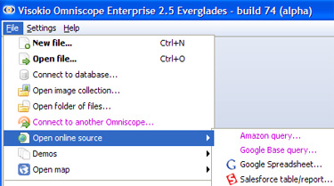 | 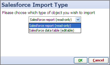 |
Once you have successfully logged in to your Salesforce account, you can choose to import either an existing standard or custom Report data set, or an existing standard or custom Data Object. Report data sets can be configured, saved and shared with others, including additional data merged in from other non-Salesforce sources. However, copies of the data in Reports files cannot be edited offline such that the changes are synchronised back to Salesforce. Un-joined Data Objects contain many fields (columns) which can be filtered and corrected offline in Omniscope, and the changes synchronised back to Salesforce.
Note: some fields (columns) in every Data Object are Salesforce system-generated and cannot be edited offline. In addition, some records (rows) in Data Objects/Tables which have become interconnected with other Data Objects/Tables, such as converted Leads, cannot be edited/synced back to in their original Leads Data Object/Table, but the user-editable fields related to unconverted leads CAN be edited and the changes synced back to the Leads Data Object/Table.
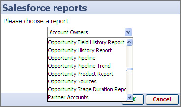 | 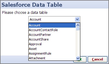 |
Use Omniscope to filter records (rows) for blanks, variations in spellings, inconsistencies among different records relating to the same account, and other typical data quality problems. Make systematic corrections, even across thousands of records, very quickly and easily in Omniscope, then synchronise the changes with Salesforce (see below). Regularly archive copies of all Reports and Data Objects/Tables. Quickly perform data integration by merging in data from other systems and/or stand-alone or collaborative spreadsheets.
If you open an online Report or Data Object/Table for the first time using the direct connector in Omniscope Professional 2.5, you will have to configure the Omniscope file report tabs yourself. However, if you have installed the free Omniscope (web) Connector for Salesforce [512]in your account(s), you can download an existing templated file for each standard Report or Data Object/Table from the 'Visokio Reports' tab, then follow these directions to change the file data source [526] so that you can start from an already templated reporting file. Once you have fully customised your copy of the pre-templated file, and synchronised any changes to the data with Salesforce, you can upload the file back to the Visokio Reports tab, adding a new, customised template download option for each Report or Data Object/Table. Colleagues will be able to download future fresh views of the data using the now customised template, even with the free Viewer.
Note: Uploading a populated customised file to the 'Visokio Reports' tab as a new template does not synchronise the data. Only the layout, report tab configurations and overall look and feel of the file is remembered. Each future download is fully re-populated with the freshest data from Salesforce.
Once you have downloaded and added to or edited user-editable fields (columns) in Omniscope, you must synchronise these changes with Salesforce in order for your changes to become persistent in the online data. When you are ready to commit your changes to the online version of the Salesforce data, go to Data > Synchronise with Salesforce to launch the synchronisation wizard.
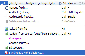
WARNING: If you close and open your local Omniscope file before you have successfully synchronised with Salesforce, be sure to skip or cancel the refresh, since this will overwrite any changes you made in the local file with values from the current online data set. You can avoid this risk by saving local copies with un-synchronised changes with the refresh option set to 'Never' until all changes have been successfully synchronised.
The Synchronisation wizard opens comparing the status of your local Omniscope version of the data with the then-current version of the Data Object/Table downloaded in Salesforce. In the example below, no new rows were added online while the file was being edited locally in Omniscope. Had new records been added by someone else online, they would show on the right current Salesforce pane in green, with the option to download the new records (rows) during synchronisation.
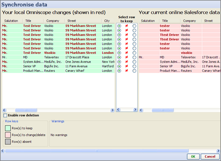
By default, there is a protective setting preventing online records from being deleted if they are not present in the local Omniscope copy. To change this, tick the option to Enable row deletion below the local changes listing.
More detail on synchronisation [527], best practices and common warning and error messages.
You can save time configuring Omniscope files for all your Reports and Data Objects if you start by downloading a copy of your data using the default templates available on the 'Visokio Reports' tab of the web connector tab for Salesforce, a certified, free AppExchange-listed application [512] your Administrator can install.
The templated files available via the web connector are downloaded without a linked source. To add/edit and synchronise data saved locally in Omniscope with your online instance of Salesforce, you first need to associate each downloaded file with the corresponding Salesforce online Report or Data Object directly.
Changing the linked data source of a file is done from Data > Change source by selecting select Salesforce importer as the type of data source.
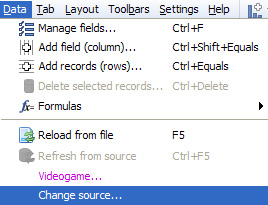 | 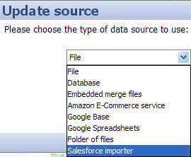 |
If you are working with a downloaded Report file, and are interested in live refresh of the data in the Report file, choose Salesforce report. The data in Reports cannot be edited directly, but can be refreshed on demand into Omniscope, and the configuration of the Omniscope file changed and saved/forwarded assuming you have an activated edittion of Omniscope (not the free Viewer).
If you are working with a downloaded Data Object/Table, and you wish to add/edit data then synchronise the changes with Salesforce, choose Salesforce data table, which are editable. You will then be prompted to login to your Salesforce account and asked to paste-in your security token. Note: Salesforce Group accounts do not support direct connections.
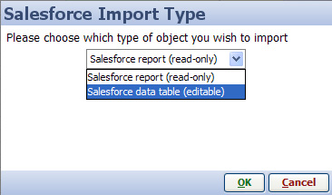 | Please note: Some fields (columns) and some records (rows) within each Data Object/Table are not directly editable from outside of Salesforce. They may need to be edited from inside the web interface of Salesforce, or by reference to another Data Object/Table. Fields which are not editable are indicated in the heading. Rows which are not editable are usually screened out by filters set in the editing tab of the default template. |
{in progress}
Omniscope 2.5+ provides a connector that allows you to download data from Facebook. Using the Network View, you can visualise the interconnections and relationships in your Friends list.
To import data from a Facebook account, select File > Open online source > Facebook.
| First, you must click on the link at the top of the dialog. This will take you to the Omniscope Facebook connector log-in screen. Enter your Facebook username and password and click 'OK'. Tokenise friend list - adds a separator beween each friend and enables Omniscope to treat each friend as tokenised text [419] Show user profile images - |
All options to import data present in Toolbar menu are the same options present in DataManager. Click Here [397] for more details. One Option has been Added: Open map This option allow the suer to Add Online Map: For more details of how to use Online world click Here [401]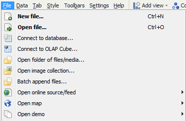
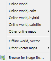
You can create a new Omniscope file 'from scratch' by entering data into the Table View, much as you would with a spreadsheet.
Populating data (brief guide) , Links to Editing topic,
Omniscope types uniformly empty (null) fields as 'Text'
Converting fields => Configuring data sub-topic
Omniscope can open most common delimited data files and tagged XML files suitably transformed. Clicking on File > Open file brings up the Open file dialog, which looks similar to a Windows file browse dialog:
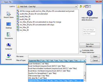 | File > Open dialog: Most source data files in Excel XLS, CSV, TSV and other common delimited text data file formats will open directly in Omniscope. The Help icon in the upper right displays a format guide [528] for importing spreadsheet files. Always confirm that your spreadsheets conform to this simple layout before trying to open them in Omniscope. If you have problems, such as all the values appearing in one column, you may need to change the delimiter or rename a tab-delimited file extension from TXT to TSV. If only some of the data fields (columns) have not separated cleanly, you can use the Expand or Collapse Values functions in the Table View Tools [3] menu to separate data into more columns or combine data from multiple columns into fewer columns. If you encounter problems importing data from one or more files, see also the KnowledgeBase section on importing and exporting data to and from supported data files. [473] Note: Importing XML files requires that the file be transformed to a single tabular structure in our schema (see below). |
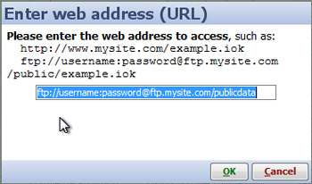 | Opening remote data files over the web -
|
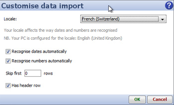 | Adapting to regional and non-standard data formatting - If you are repeatedly using/importing other peoples' spreadsheets, you can depart from the recommended standard spreadsheet layout somewhat by ticking the Customise data import behaviour option and providing Omniscope with additional information about the layout of the data you are importing. For example, sometimes you may have a CSV, TSV or Excel XLS file which does not have the column headers on the first row. Without customisation, Omniscope will assume the first row contains headers, and include the actual column headers as the first row of data. To skip any number of redundant upper rows on file import, use the Skip first ?? rows box to enter the number of redundant (usually formatting) rows in your data file to be skipped before trying to read in the headers. |
Data File delimiters - the CSV file extension stands for "Comma Separated Values", which means the cells in each row of the data table are separated by the comma character. However, if you are in a region that also uses the comma for the decimal point (e.g. several European countries, such as France) some versions of Excel create CSV files that use a semicolon as the separator character. Sometimes these files are saved with a TXT rather than CSV extension, even though they are multi-column tables. Omniscope is unable to detect these situations automatically. If you open such a file in Omniscope, your data will very clearly be wrong, with most columns appearing as text with semicolons. To import this kind of file, use the Customise data import option dialog to change the Separator character to a semicolon " ; ". Pipe "|" delimited files can also be imported, but first you must re-save the file with a CSV extension, then use the option that appears to change the delimiter to "|".
Dates & Numbers - if you are running on Windows, when importing data that is in a delimited text format which includes Excel, CSV and TSV (tab-separated values), Omniscope will use your Windows Regional Settings to try to automatically recognise data. For example, for a PC with United States Regional Settings, Omniscope will recognise "5/13/2005" as a date and "1,500.5" as a number. For some international users, however, this may not work as expected and the result will be an import of all columns as type Text (shown either as multi-coloured Category columns or white Text columns in Omniscope). If this occurs, you can usually manually convert numbers and dates & times fields using the Data > Manage fields dialog. for more information on formatting dates & times, and dealing with time zone issues, see the section on Dates & Times.
If you know your data has been formatted for a different region, change the Locale drop-down accordingly. For example, if you live in Germany but have received a CSV from an American customer, you should choose 'English (US)'. If you find Omniscope gets things wrong and your data is incorrectly recognised, you can disable auto-detection of dates and numbers by deselecting the two Recognise...checkboxes. All fields will open as Category or Text data and their text values will be preserved. See the KnowledgeBase section for more on information on dealing with International data issues. [529]
Importing XML files which have already been transformed to Visokio XML Schema [472] is the same as opening a CSV.
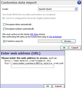 | Transforming XML into Omniscope Schema - If your XML file conforms to another schema, then you must prepare an XSL Transform [530]file, tick Customise data import and specify that file to transform the non-Visokio XML file to Visokio XML schema for import. Your XSL Transform stylesheet can be accessed from any location, including the web, using the Enter web address (URL) option to specify the online location of the XSL file.
Note: if your XML data set is not already in a tabular structure, you must array it into a tabular structure using your XSL file.
|
Omniscope DataManager workspace currently supports direct connections to Microsoft Analysis Services and some other MDX-compatible mutli-dimensional cube structures from other vendors.
MS SQL Server Analysis Services (SSAS) example [531]
Recent versions of Microsoft SQL Server 2008 includes Reporting Services (SSRS) and Analysis Services (SSAS).
Same as file metadata
Omniscope can treat any folder (and related subfolders) containing files as a data source using the File > Open folder of files/media connector. Omniscope asks for a starting folder, and will scan all files within the folder, representing each file as a record within the resulting data set. When Omniscope opens, you will see fields and corresponding filters realting to all the attributes of the files in the folder(s) - filenames, extensions, category, size, date, etc.
All supported media files will have not only their filenames but also their tags imported as additional columns. For example, the ID3 tags of an MP3 file, such as Artist, Album and Track Number will be imported, as will the meta data in a JPG photo file, including camera model, date taken, and geo-location (if available in the file). Tag fields will be available as Sidebar filters where commonly useful.
After import, Omniscope will show default Pie and Tile Views illustrating the types of files you have (such as audio and image), and a Table View showing the data, including colour-coded table headers for tags. The Tile View will also display the images for any image files.
Include subfolders - by default, this is ticked, meaning all subfolders and sub-subfolders (etc.) of the selected scan folder will also be processed. If unticked, only files directly in the selected folder will be processed.
Include files without extensions - by default, files that do not have a dotted extension such as ".txt" or ".jpg" are excluded. If ticked, files without any extension will be included. On Windows machines, most files already have extensions.
Customise which file types are included - by default all files are included. Tick this option to provide a comma-separated list of extensions to permit such as "jpg,mp3". All other files will be skipped.
Tags in filenames - you can also choose to include "Tags in filenames" from in the file chooser when browsing for a folder. This will prompt you to define the "Filename structure", which is the format of the filename as a series of delimited values, typically using a hyphen to separate them. Omniscope will then read each filename tag as an additional column. For example, you might standardise on naming your photo files according to the convention "1983-Paris-Jim's wedding", in which case you would use the format "YEAR-LOCATION-DESCRIPTION" and Omniscope would then create 3 editable fields accordingly.
You can edit the tag columns (shown in the Table View using colour-coded headers) like any other values in cells. Then, use File > Export > Apply tags to files to save your changes back to the individual files where they are stored. All filename tags will be applied (which will physically rename your files), but only supported media tags such as MP3 Artist will be applied. A comprehensive list of supported media tags for reading and writing is shown in each table column header's tooltip displayed by hovering your mouse over the column header.
Warning: The following text/screenshots apply to earlier versions of Omniscope and may be slightly out of date.
Opening a folder of files is similar to opening a folder of images. For example, Omniscope can be used to explore folders of files on part or even all of your PC or connected servers' hard disks. You can also use Omniscope to manage media file libraries (Audio, Video and related Images) including powerful options to modify and harmonise Tags as well as file naming conventions.
Choose File > Open folder of files/media. Browse to the top-level folder you want to explore (for example your entire C:/ root) and click Select. After a few moments, depending on the number of files scanned, you will see a Pie View on the left, a Tile View on the right and the right-hand Sidebar with filter/query devices showing both file attributes like Extension, Category and Size, as well as Tag: values. The Pie View is initally set to show the distribution of files by Category, whereas the Tile View represents each file as a tile, initially grouped by types of files (System files, Video files, Music files, etc.) and sized according to the size of the file. On opening, colour is used to show the date of each file. A green tile represents a recently modified file; red represents older files.
This view allows you to see at a glance where the space on your hard disk is allocated (by the size of the tiles), what sort of files they are (by the grouping) and how old the files are (by the colour).
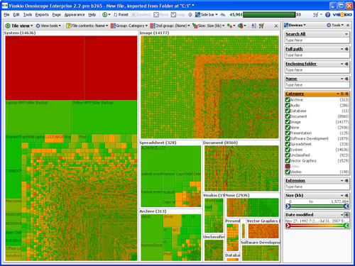
The smallest tiles/files might not be clearly visible if they are much smaller than the biggest files. Use the Side Bar query devices on the right to filter and search for relatively smaller files. For example, on a Windows machine, certain very large system files have very old dates. Filter them out by excluding System files in the Side Bar. You may want to do the same for Video files. Now set the 2nd Group option to Enclosing Folder, enabling you to see the exact locations of your larger, older (non-system) files:
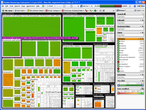
You can change the primary grouping (using the Group drop-down in the Tile view) to show Level 1, which groups the files according to the first level of folders in your directory structure. You can also change the 2nd Group option to Extension to gain an overview of your files by file type. After you have analysed your Images, for example, exclude them using the Side Bar filter to focus on other types of files which tend to be smaller. Instantly you will see the relative size of each top-level folder, excluding System, Video and Images.
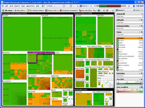
By filtering out all files that are not documents, you can use Omniscope as a document browser. For example, the Web View can display any Acrobat .PDF document. Saving this configuration as a Report Page with the filter set to Documents only permits any recipient of the file to browse the documents in a defined location (any network-accessible file server, not just their local machine as in this example).
This allows you to use Omniscope to explore and manage your photo collection. Using File > Open image collection, Omniscope will ask you for a starting folder, and will scan all images within the folder, representing each as a record within the resulting data file.
You will see a Tile view showing your images in a grid, a Table view showing the data, and a series of filters. The data and filters will include information about each file, including image tags such as width, height and GPS location (lat/lon, if available).
Opening image collections is very similar to opening folders of files. See Open Folder of Files [411] for more information about advanced options, tagged files and renaming / applying edited tags to files. The only differences between the two are:
Additional advanced options
Assume files without extensions are images: By default, only files with a supported image extension (such as ".jpg") are included. If this is ticked, Omniscope will also assume files without an extension are images also. Used for specific image servers which don't provide filename extensions. All image files on Windows usually have an extension.
Warning: The following text applies to earlier versions of Omniscope and is out of date.
Omniscope can be used as a photo browser, allowing you to explore and manage large folders of images, and to send selected, annotated collections to others in compact, searchable .IOK files with supplementary information on the photos, their locations etc.
File > Open Image Collection opens a new Omniscope file in folder browser mode that allows you to point at any folder (with or without sub-folders) containing image files in .JPG, .GIF. .BMP, or .PNG format. Browse to the folder, select it and click Select.
Wait a few moments for Omniscope to import the pictures. The Tile View and left Side Bar will appear, with the images scaled down to display in the Tile View. The Side Bar filter/query devices allow you to Search All for a keyword, to filter the size of the files (and hence the quality/size of the picture), and to filter the date of the pictures. The Tile View initially shows all the pictures found in the folder chosen. As you filter, some pictures will disappear, and the remaining pictures will get bigger.
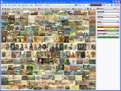
At this point, you might want to save a new .IOK file linked to this image folder. This will capture any settings you configure to the file. You do not have to embed the pictures in the file at this time. In future, you can use File > import into current file > Refresh from source to update the file to include any new photos added to the folder.
You can Select and Move pictures you want to exclude from further consideration, thereby enlarging the remaining pictures. When you see a picture you would like to add to a collection file (such as your 'holiday highlights'), click the picture to get the Details pop-window showing a larger view, then click Add to basket to save that picture in the BASKET universe. Carry on filtering and exploring your photos, adding more pictures selected for the collection file to the Basket.
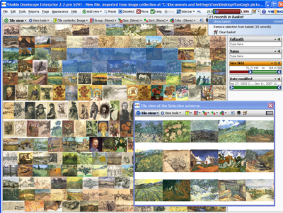
When you've finished selecting photos for the collection file, view the Basket by clicking the ![]() Basket button to the right of the Barometer on the Main Toolbar. A Table View of the BASKET universe will appear. Click Table View to display the View Chooser, and select a Tile View of the BASKET universe. For more detail, see Data Universes [38]
Basket button to the right of the Barometer on the Main Toolbar. A Table View of the BASKET universe will appear. Click Table View to display the View Chooser, and select a Tile View of the BASKET universe. For more detail, see Data Universes [38]
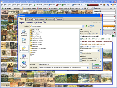
If you're happy with your BASKET of images, you might want to view a Slide show. See Viewing Details [66].
When you've finished reviewing the images you wish to save as a collection, choose File > Save as IOK/IOM. In the Save as dialog that appears, you will see a number of configuration options on the right-hand side.
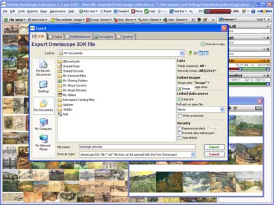
Click Records (rows) and choose Records in the Basket (XXX records). This will create a new file with only the images you added to the Basket. When you make this change, the dialog will transform from a Save as dialog to an Export the images [532]dialog with the Images tab pre-selected.
Under Embed images, click Image sets and tick Image. This means the image set called 'Image' will be embedded inside the IOK file. In other words, the IOK file will be like a ZIP or archive, containing images. If your images are quite large, you may want to down-size them when embedding in the IOK file. If so, tick Reduce image sizes. A dialog for down-sizing the images will appear after you click Export. In Linked data source, un-tick Keep link to remove the reference to the original folder of images on your PC. Enter the name you want to save the file as, say 'My holiday snaps', and click Export.

If you chose to reduce image sizes, enter the maximum dimensions you want for any image (in pixels), and all images exceeding these dimensions will be down-sized, preserving their aspect ratio, until they fit within these dimensions. You may have to wait a while down-sizing the images, but once done, you should have a simple and small (depending on the size and number of images) Omniscope file for sending to friends.
If you send an .IOK file, they only need the Omniscope free Viewer to open and view it, even export their own selected images if you have not locked the file.
Visokio supply zooming vector maps you can include in your files. Vector maps work offline, and zoom to show detail, although not down to city street level. If you send the file to someone who does not have the vector map already installed, it will be downloaded when they open the file, even if they are using a free Viewer or Omniscope Online [396], the 'zero-footprint' Java Web Start deployment of the Viewer.
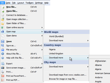 | World maps: these maps cover the whole world World (bundled) - every Omniscope contains a vector world map, but additional world maps can be added to any installation or file via download. Country maps: we offer a complete library of geo-coded country maps. Maps already installed will be listed, with more available for download. City Maps: we are in the process of adding geo-coded city maps to our library. Contact [86] us for the city you need. Alternatively, you can use static image screenshots from street-level mapping services like Google Maps (see below). Download maps - takes you to the Maps Library Browse for image or map file - any image can be used as a mapping background, and coordinates consistent with your data can be added to the image. The imported image file becomes embedded in the Omniscope file/DataPlayer and travels with the file. |
For more information on adding coordinate systems to imported images and screenshots, i.e. street level screenshots from Google Maps, etc. please see the KnowledgeBase sections on Using Maps [533] and Projection Transformation [59]
{in progress}
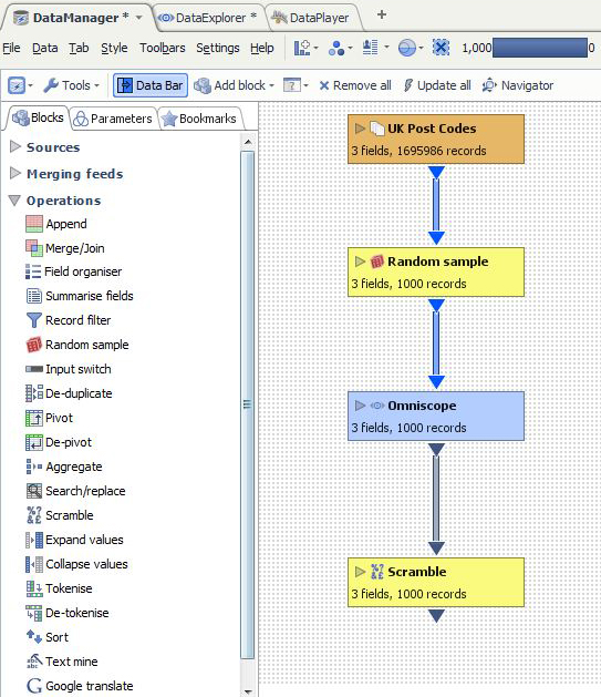
Operations blocks are managed similar to source blocks, either dragged from the Data Bar or added from the Add Block View Toolbar drop-down menu.
Omniscope is a very powerful visual tool for detecting and 'scrubbing' errors and making changes to your data. Once you have imported all the 'raw' data from various sources, you can use Omniscope to ensure the completeness and correctness of the data following the Data Management phase checklist [467]. Topics:
Editing Cell Values [417] - the Table View permits you to edit values in data sets at individual cell, value or column level using familiar keyboard shortcut commands
Rows & Columns [418] - adding and deleting rows and columns, setting column orders, configuring row height etc.
Dates & times [110] - specifying and changing the format of data stored in your source files as imported Omniscope date & time values.
Note: Omniscope does not currently support time durations as data values. If you are managing time durations, you must either import start & stop times & dates and let Omniscope calculate durations, or use and display durations as decimal numbers, e.g. 3.5 = 3 hours and 30 minutes
Tokenised data [419] - using data sets with more than one value (or image) per cell, i.e. one to many relationships in 'flat' data sets
Time Series [420]- Omniscope stores repeated observations over time as rows (not columns). Consult this section if you plan to create time-series displays from your data set.
Placing markers [422] - Omniscope enables you to add or edit geographic coordinates associated with a map manually. Use this approach to check your geographic coordinates, add missing coordinates, and refine the coordinate columns in your data set by referencing highly detailed online mapping resources such as Google Earth/Maps.
Data entry - see the Details View [20] to learn how this view can be configured as a data entry screen and added to any tab. Use formulae fields to set validations, and use Source IOK visualisations to 'flag' invalid inputs. Export/post edited data as corrections files/tables using web services and other methods.
Keyboard shortcuts [448]
WARNING: Depending on your data source(s), you may or may not be able to directly write-back or synchronise your changes with the linked source of your file, such that your changes will survive future file data refreshes (see below). In the case of direct database connections, we do not recommend writing manual changes directly back to the relational source tables. However, unless you follow an agreed manual corrections file export/import procedure, the next time you refresh your Omniscope file from its database source, some of your data edits could be replaced with the as yet uncorrected contents of the source database.
Use the DataManager workspace to specify changes to data pending correction of the data in the source databases. This will ensure that your changes are repeatly applied on each refresh/recalculation, ensuring that Reports are always correct even if the source data remains uncorrected.
To preserve data not contained or being corrected in the source database, you can divide your data set into two parts, one Source IOK file with the same fields as the database and that refreshes directly from the database, and another IOK merge file that holds your local data as edited. Following each refresh, the merge will be repeated, preserving the local data held in the IOK merge file from being overwritten by blank columns from the database refresh of the Source IOK file.
Omniscope is a powerful tool for editing the values in data sets at individual cell, value or column level. Omniscope displays cells for editing in the Table View. To edit the value in a cell, point the mouse at the cell in the place where the edit begins and double left-click on the cell and the cell will open for editing with the cursor placed where the edit begins. You can also use Right-click on cell > Edit this cell and the cell will open for editing with the cursor placed at the end of the cell.
Each Omniscope cell can contain an unlimited amount of text. Depending on the Row Height [418]selected, the cell will expand to allow you to read many lines, but you cannot scroll down within a cell. Keyboard shortcuts below are used for this and other basic editing operations within cells, and to cut and paste values between cells.
Note: it is not possible to edit cells if the file has been locked by the owner, the column has been set to Read-only, or Aggregations are being applied on the tab. If Aggregations are being applied, open another Table View and perform a Keep of the aggregated rows you wish to edit to make the aggregated records visible in the Filtered data IN data subset, and therefore editable in the non-aggregated Table View.
The following keyboard shortcuts are used used to speed editing of cells, copy & pasting values into other cells down many rows or across many columns and navigation of cells containing many lines of text:
Alt+Return adds a line return inside a cell containing text
Ctrl+A selects all the text in the cell
Delete deletes all selected text
Backspace deletes selected cells or text
Ctrl+C copies the selected cells to the clipboard
Ctrl+V pastes the values in the clipboard to the selected cells (see warning on large pastes above)
Ctrl+X removes the current values from the selected cells and stores them in the clipboard
Ctrl+Z undoes the previous edit
Ctrl+Y re-does the previous undone edit
Ctrl+; inserts the current date into the cell
Ctrl+End moves the cursor to the end/bottom of the text in the cell.
Ctrl+Home moves the cursor to the top of the text in the cell
Page Down moves the cursor a full page down the text
Page Up moves the cursor a full page up the text
Note: Macs use the Command key instead of the Ctrl key. See the full list of keyboard shortcuts [448]
You can move data into or out of Omniscope using copy and paste (assuming the file owner has not locked the file). Column headers are used to set sorting behaviour and cannot be used to select an entire column. To select most or all of a long column, hold the Shift key down and drag the right Table View scroll bar to the very bottom of the target range. Then click on the last cell in the range so that all intermediate cells will be selected and become targets for edits like copy & paste and delete.
WARNING: Be careful when pasting large, rectangular tables of values into Omniscope. If you specify a target paste range with more rows and columns than are contained in the data set you are copying, Omniscope may duplicate the records to fill the target space entirely. If you are not sure how many rows and columns you are importing via copy and paste, create a large number of new rows and columns and select only the single upper left-hand cell as the target paste range. This usually pastes the correct range. However, depending on the format/source of the incoming pasted data (web page tables, for example) all of the incoming values are sometimes pasted into the single upper left cell only. If this happens, then you must specify a rectangular target area exactly the correct size to receive the incoming pasted data. If you accidentally make the paste range too large, be sure to check for, and delete, any duplicated records.
There are two different ways to make changes to multiple values in a given field (column) such that all instances of the value are changed; either from the Options sub-menu for the corresponding field (column) in Main Toolbar: Data > Manage Fields [31], or, if the field is typed 'Category', you can edit the category values directly from Sidebar devices by right-clicking on the value you wish to edit.
A powerful search and replace option that will work with all data types is accessed from Data > Manage fields > {column} Options > Replace within values
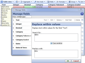 | Replace within values - this option is not global, it only operates on the specified field (column) to search and replace full or partial matches automatically. Use this tool, for example, when date formats are not consistent within a given column, and the data format needs to be made consistent before Omniscope can apply Date & Time typing. You can use this tool with Text, Category, Numeric and Date & Time data. |
If the value to be edited is in a column typed Category, you will also see an editing option from Data > Manage fields > {column} Options > Value Order,...> Edit Value as shown below:
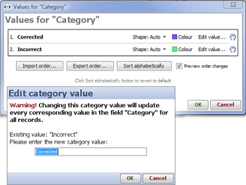 | The Manage fields > {column} Options > Value Order..., dialog enables you to change the sort order, colour and shape assigned to each Category value in the column (see below), as well as edit the values and their sort order: Edit value - replaces the selected category value with the specified text for all rows in the specified field (column). Once you have corrected all values in the Category column, use the 'hands' to change the sort order by dragging values upwards or downwards. This top-to-bottom sort order will be used throughout the file, for example in the Sidebar category filter devices, etc. You can export and import long sort orders e.g. bond ratings as text files and revert to the default alphabetical sort order at any time. Ticked by default, the Preview order changes option allows you to see the effect of order changes immediately.
|
Specific values in a category field (column) can also be edited collectively directly from the Sidebar, as can the colour and shape assigned to each category value:
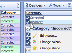 | Right-clicking on the value to be edited displays a drop-down menu from which the value can be edited, as well as the colour and shape assigned to the value changed. Clicking on Edit Value will display a warning and a field where you can enter the corrected value for rows whose column values you wish to change.
|
Because Omniscope has features of both databases and spreadsheets, the terms 'columns' and 'fields' are interchangeable, as are the terms 'records' and 'rows'. Omniscope imports tabular data sets which are structured into fields (columns) and records (rows). The default opening Table View provides a traditional, tabular 'row and column' view of the data set in the file. Current versions of Omniscope assemble all imported and merged data into only a single table, but future versions will be multi-table.
You can add fields and add and delete records from various menus, depending on the degree of control you need an where the records appear in the data set.
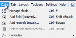 | Add field (column) - adds a new named column to the data set at the far right of the columns in that Table View, and the bottom of the list in Manage fields. Add records (rows) - adds a specified number of blank records to the bottom of the data set display. Delete selected records - displays warning asking if you want to permanently delete the records currently selected. |
The left-most, unlabelled, narrow column in the Table View is the Row Header. Left-clicking on the Row Header selects that record. Hold down the Ctrl key and you can select any pattern of rows. Double-clicking on a Row Header displays the Details for that record according to the Details display settings available from Main Toolbar: Settings > Details. Right-clicking on a Row Header, or selected group of Row Headers, displays options for adding, deleting and duplicating rows:
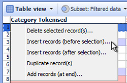 | Delete selected records - displays warning asking if you want to permanently delete the records currently selected. |
Note: When adding or deleting rows, make sure that the Table View you are using is displaying either the default Filtered data (IN) subset with no records filtered out, or better yet the All data subset. This ensures that the new records (rows) are not subjected to filtering and named Query settings until fully populated.
You can change the ways rows are displayed from the Table View: View Tools > Row options menu:
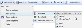 | Row title - by default, Omniscope displays a record number in the Row Header sequenced as in the data source. You can save space by selecting (None), or choose to substitute this with values from a column in the data set (usually one with complete and unique values), which can then be hidden |
Show link shortcuts - by default, the far right end of each row displays a links menu providing links related to the record, a list of pre-configured links that may suit some fields in the record, and options to create both local and web links. If no links are configured in the file, only the Details link will display. You can choose to hide the link shortcuts in any given view by toggling the Show link shortcuts option. See Creating links [534]for more detail.
The Add new field button at the bottom of the Data > Manage fields [31]dialog enables you to name and add a new filed, but you must then drag the column into the correct column order. New fields are typed 'Text' by default
You can also right-click on a Column Header to access many column-related commands with more control over the placement relative to existing column orders:
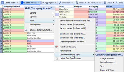 | Right-click {Column Header} > Tools: |
Delete field from data set - after a warning, permanently deletes the column from the data set. This is a remembered action that will be repeated on each refresh.
WARNING: Be careful when clicking on Column Headers. Unlike spreadsheets, a left click on a Column Header in Omniscope sets a Sort...see Setting & Clearing Sorts)
To select most or all of a long column, after selecting the first cell, hold the Shift key down and drag the right side Table View scroll bar to the bottom of the target range. Then click on the last cell in the range so that all intermediate cells will be selected and become targets for edits like copy & paste and delete.
Omniscope makes use of repeated observations over time in vertical rows, rather than the horizontal column layouts often used to lay out spreadsheets. To create a multi-line time series in Omniscope, put your data in a 'vertical' format like that illustrated below, where each successive record in the data file is a price observation for a company's shares at a different point in time:
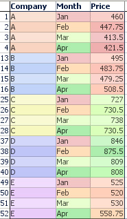 | In this example of a time series, we have 5 companies "A" to "E" with historic share prices for each month. The Company field contains Category values correlating to different lines in the time series. Let's call this our Category field. The Month field contains Date and Time values representing the time part of the time series, along the X axis. Let's call this our Time field. The Price field contains quantitative Decimal number values for the Y axis. Let's call this our Value field. Don't worry about the vertical repetition in the data...this will be invisible in all views except the Table View and not evident in the time series reports you configure. |
Check your data types - After importing your data, make sure the Time (here Month) and Value (here Price) fields are the correct format. They must be numeric (decimal or integer), or dates, shown by the red to green colour gradation. Also make sure the Category field is of type Category, shown by the variety of different colours. You can convert data from one type to the other by right-clicking the column header in the Table View and choosing Convert field data type.
Sometimes time series source data is laid out horizontally (repeated observations in columns) when Omniscope would manage it better vertically. In other cases, data may need to be exported from Omniscope in an orientation different from that used in the Omniscope file. To avoid the time consuming process of changing the orientation of some or all of the data from horizontal to vertical (row becomes column) or vertical to horizontal (column becomes row), Omniscope has both De-pivot and Re-pivot functions. Use of these functions is discussed here [41].
For a continuation on displaying line graphs like time series, see the the Graph View section displaying time series [8].
You can use embedded vector maps or online Google Maps from within Omniscope to add map coordinates to your data by selecting records (rows) and manually placing markers on an open Map View.
To place markers and automatically generate coordinates in your data for existing records (rows), open your data set and close all open views except:
These views must be open simultaneously, and you might want to drag or switch (rotate) the view divider to allocate more space to the Map View. When you add the Map View, if this is the first time you're adding markers to the map, you will see the Configure Map dialog asking you to configure the map:

Make sure Add new X/Y field pair is selected, and click OK. You will be able to name the new. blank coordinate fields in the dialog.
Suggestion: name the X-axis with something related to longitude and the Y-axis with something related to latittude.
Next, filter your data until only the records you want to place to generate coordinates remain visible. For example, if you have already placed some markers, you will want to filter out the records that already have coordinates. This will make focusing on the remaining records with blank coordinates easier. In the Omniscope Table view, scroll across to the coordinate fields, and click on any grey (blank) cell. This will select all the records without coordinates. Click Keep on the Main Toolbar to isolate only those records in the Table View.
In the Map View, first make sure Place marker mode is selected in the mouse Mode drop-down.
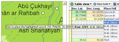
Notice that the X and Y coordinate fields visible in the Table View are populated automatically with latitude and longitude coordinates when you do this.
Sometimes you might want to place a range of records at a single point on the map. For example, you might have a database of customers, and you might only know they are based in London. In the Table or Chart Views, select the records you want to place in the same location. In our example, there might be a field called 'Location'. In the Chart View, we would open the Location device and select the value 'London'. In the Map View again, still in Place marker mode, point at London and click to place all selected markers in London.
After zooming in and exploring your map and markers, you might want to adjust the position of some of them. In Place marker mode, dragging a marker will update its position. If the marker represents several records, only the top-most record in the "pile" will be repositioned.
When in Place marker mode, if you click on the map without record(s) selected/highlighted, you will be asked if you want to Add a record at that location. This will create a new record (row) in the data set, with all fields empty except the coordinates.
Once you have successfully imported your data, and confirmed that you can refresh from the original source(s), you can follow the Analysis phase checklist [468] to optimise your file. Most changes you make to your file are remembered and re-applied when you refresh the data from source, but not all. Changes which will not survive a refresh are noted, and you must follow a source data correction procedure that depends on the nature of your sources. Omniscope can write changes back to data files such as a spreadsheet, but this is not currently supported for direct database connections. Some connectors, such as the Salesforce direct connector, feature synchronisation of changes with the live source online.
Manage Fields [31] -
Setting & Clearing Sorts -
Formula Fields [30] [30]- You can define Formula fields (columns) to be evaluated according to mathematical functions and logical expressions using the values in other columns. In addition to the same functions used in most spreadsheets, Omniscope also features powerful SUBSET functions that operate on entire data sets. This section introduces the use of Formula fields (columns) and provides links to more detailed sections on defining your own formulae and using Variables (assumed values used for sensitivity analysis) with links to the Functions Guide [137], which provides detailed documetation and examples of commonly used formulae.
Omniscope gives you many options to use colour to communicate more about your data visually.
PENDING: global and per-view colouring, and precedence; how colouring of elements representing multiple records uses averages; links to configuring value colouring options and other colour-related options e.g. in the table view
Once you are satisfied with the content of your data set, you are ready for the next phase of file preparation following the Visualisation Phase checklist [469].
Selection
Filtering
Queries & Subsets [22]- Introduces the related concepts of Named Queries and defined data subsets. The Main Toolbar Named Queries menu options are covered, as is the Data Subsets selector that appears on most View Toolbars immediately to the right of the view name for all views.
Aggregation [425] -
Using an activated Omniscope, you can add a new view to a tab, or change a view from one view type to another, at any time using the Maintoolbar: Add View icon drop down to dislay the View Chooser, or clicking on the far left view icon on any view toolbar, which also displays the View Chooser
Applies to verison 2.4 only;
Omniscope 2.4 offered 14 different views, but version 2.5 has expanded this to 16, with the former Tree View being replaced by the new Network View. You can use these views in any combination to help you and recipients of your files analyse and illustrate the messages in your data. Omniscope views offer much more than just data visualisation and portable/exportable charting and presentation. Most views are complete data navigation environments enabling browsing, aggregation, analysis, filtering and drill-down to details. All views set to show the same data subset/named query e.g. 'Filtered data (IN)' or 'Errors for Correction' update simultaneously to reflect filtering actions.
![]() on the Main Toolbar displays the vertical View Chooser drop-down menu. The same display can be use to change a view window from one view to another by clicking on the left-corner view icon on the View Toolbar. On the View Chooser, each View is represented by its own icon:
on the Main Toolbar displays the vertical View Chooser drop-down menu. The same display can be use to change a view window from one view to another by clicking on the left-corner view icon on the View Toolbar. On the View Chooser, each View is represented by its own icon:
Click on the view icons above or the names below to go directly to the discussion of each individual view:
|
*To see the experimental views available in your version, tick this advanced option, then re-start your Omniscope:
Version 2.4: Tools > Advanced Tools > Application wide settings > Show experimental features;
Version 2.5: Settings > Advanced > Show experimental features.
Some of the views are slightly different:
Web View [16] - opens browser window(s) showing linked web pages and the results of web services associated with the data set.
Content View [18] - displays free text commentary and links to web assets, including images and charts not referenced in the data set
Dial View [19] - creates typical dashboard-style gauges to display field (column) composition, progress and alert conditions, etc.
Details View [20] - displays all (non-hidden) values for each single record, together with images and buttons/links connecting to related web pages/services.
DataPlayer View [427] - allows anyone to create interactive Flash DataPlayers encapsulating the data in exportable 'dashboards' for documents and web pages.
If you wish to arrange more than one view on a tab, you can control the amount of space and the order of each view.
Immediately to the right of the Help command is the Add View drop down menu, used to add an additional view to the current display. To remove a view from the display, click on the [X] in the upper right hand corner of the view. To change a window from one view to another, click on the view name and select the view you want from the drop-down menu. If you want to add a view showing another data subset, you can select it using the Data Subset drop-down to the right of the view name in each View Toolbar.There is no upper limit on the number of views you can open in Omniscope, but display screen size limitations encourage using multiple tabs to display different combinations of views, rather than crowding the working display with too many open views.
Hint: It is best to first create a layout of view windows the right size and shape for each view, then switch each window to be the desired View. Easier than Rubik's Cube!
In addition to the Main Toolbar barometer, many views display view-specific barometers whenever they are displaying a data subset different form the Filtered (IN) subset.
Options for each view are generally available on the View Toolbar. Many of the commands available from the View Toolbar > View Tools drop-down menu are common to all views. Commands or options common to all (or most) views are documented here: View Tools common commands [2].
Applies to version 2.4 and prior
Each View has a View Toolbar, which presents the features and options applicable to that View, including a View Chooser, Data Sub-Set selector, Aggregation options, a View tools drop-down menu, Fields (columns) picker and other options specific to each view. View Toolbars open and close at the top of each view window. All views and View Toolbars always open below the Main Toolbar, whose commands apply to all open views.
View Toolbars vary in appearance, since each View features different controls on the toolbar, but they typically look like this:
![]() [update to 2.4]
[update to 2.4]
In the left corner of each View Toolbar is the View icon which identifies the view currently selected. Clicking this icon also reveals the vertical View Chooser drop-down from which you can change the view shown in that window. On the right-most end of all View Toolbars is the Close View icon, shown as a black [X]. Click this icon to close the view. You can always bring closed views (or new, additional views) back by clicking this icon on the Main Toolbar:
By default, new views will open with the Data Subset selector set to 'Filtered data (IN)' meaning you're looking at all the records that meet the filtering criteria expressed on the Side Bar. You can change the Query/Subset of the data shown in the view using the drop-down selector. More on Queries & Subsets [22]
Beginning with version 2.4, many Views include an Aggregation drop-down menu, used to define aggregated views of the data, together with the function to be applied when aggregating each field (column). Aggregation differs from the presentational Grouping options available only in the Table View. Unlike Grouping, the end user is not meant to 'unroll' or 'drill down' the defined aggregation to the lower level of granularity. User-interactive Grouping can be used in addition to Aggregation. For example, a file with each row defined as an observation for a given day can be aggregated by week, then grouped by month and year. In the resulting Table View, an end user would be able to unroll the groupings down to weeks, but to see the maximum granularity daily data, they would have to remove the Aggregation settings.
Omniscope provides several ways for users of files to filter/query the data in the file.
The de-query option allows you to modify data subset definitions selectively to return records already filtered OUT to the filtered IN data set.
Relates only to version 2.3 and earlier. Data Universes have been reclassified as Data Subsets selectable using the Data Subset drop-down selector in each individual View Toolbar, and configured using the Queries drop-down on the Main Toolbar (2.4)
When Omniscope filters records, where do the excluded records go? Don't worry...they are not deleted! Based on your filtering decisions, Omniscope classifies each record (row) in a given file as being in one or more Data Universes:
All of these Universes can be viewed at any time in any of the 12 available views in Omniscope. Click on ![]() Add View on the Main Toolbar, then select the Show other data universes option at lower right.
Add View on the Main Toolbar, then select the Show other data universes option at lower right.
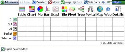
Tick the box representing any combination of Views and Universes to see the records (rows) currently in each universe in each view.
If you save an Omniscope file, the contents of the IN and OUT Universes will be preserved, and the file will open with the barometer showing the same IN/OUT split as when the file was last closed. However, the contents of the BASKET and SELECTION Universes will be re-set. Always remember to do something with the contents of your BASKET universe before you close the file, because this selection of records will not be there when you open the file again.
Let's explore the use of Data Universes in Omniscope, while re-visiting the filtering aspects of navigating .IOK files. Recall that there are 2 filtering approaches in Omniscope, which can be used interchangeably at any time, assuming at least one SideBar with instant filter/query devices is showing.:
For this tutorial, please download another, especially-configured version of the Everton Football Universes [542] file. This version of the Everton file has been configured to open with five Table Views, one for each Universe, and with only one Side Bar open:
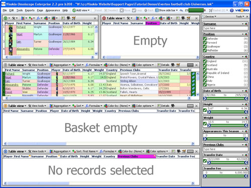
The View icons on the far left of each View Toolbar are coloured to show which of the 5 Universes is being displayed in the view. In this demo, the upper left-hand Table View is showing the green IN Universe, all 23 players. The upper right-hand Table View is showing the red OUT Universe, currently empty because no players have been filtered out. The full-width black ALL Universe Table View in the middle will always show all players, regardless of filtering. The gold BASKET Universe Table View is showing 'Basket Empty', since no players have yet been placed in the Basket. Finally, the bottom blue SELECTION Table View is empty, indicating that no records are yet selected.
Using the Side Bar, type the letter 'B' into the top text query device labelled Surname. Notice how the right-hand green IN Table View changes to display only the 3 players whose surnames begin with B, and the left-hand red OUT Table View now displays the records for the 20 players whose surname does not begin with 'B'. A glance at the barometer confirms that the green IN Universe contains 3 players whose surnames begin with B, and the red OUT Universe contains 20 players whose surnames all begin with other letters. In the Side Bar, back-space over the letter 'B' to clear the Surname query device, which will Reset the file, since this was the only extant query/filter setting.
Notice that when using the Sidebar devices, the bottom Table View showing the SELECTION Universe did not show any records being selected, and that moving 20 players to the OUT Universe was instant.
Now let's try using Selection, which can be very useful for drilling-down and confirming details before deciding whether to execute a Move or Keep operation.
Go to the upper right green Table View showing the IN Universe, and click on the Position category Defender, which will display an animated highlight in blue. This means you have selected all the players who are Defenders, and their records will now appear in the bottom blue SELECTION Table View. A glance at the barometer will confirm that you have selected 9 Defenders out of the 23 on the team.
Let's say you want to take a closer look at the Defenders. On the main/top Omniscope Toolbar, click on the green check-marked icon labelled Keep. This will keep only Defenders in the green IN Universe and move all others to the red OUT Table View to the right. Notice that the SELECTION Table View has been cleared, pending you next selection.
Let's say you want to put all the English Defenders on the transfer market (don't ask...). In the Sidebar, using the 3rd device labelled Country, click on the category name England. Notice that all other nationalities are X-ed out and all non-English Defenders are moved to the red OUT universe, leaving only the 4 English Defenders remaining in the IN Universe. Now go to the green IN Table View Toolbar, and find the Add to Basket icon right-most on the toolbar. Click the Add to Basket icon, and notice that the gold Table View showing the BASKET Universe now shows the 4 English Defenders.
Click Reset on the Omniscope Main Toolbar. This will return all players to the IN Universe, and empty the OUT universe, but leaves the 4 English defenders in the Basket, as can be seen also on the top/main Omniscope Toolbar Basket icon to the right of the barometer.
Let's save the youngest English Defender for the future. In the gold Table View showing the 4 English Defenders currently in the BASKET Universe, click on the column header Date of Birth. This will set a primary sort (see the orange downward arrow appear in the column header) sorting the players in the basket from youngest to oldest. Double-click on the row header of the youngest player, Daniel Fox. This will display the details window pop-up for Daniel Fox. Now click Remove from Basket to remove Daniel's record from the basket.
To clear the BASKET Universe completely, click on the right-most Clear basket icon in the gold Table View Toolbar, or use the Omniscope Main Toolbar Basket > Clear basket command on the drop-down menu. More on Using the Basket... [543]
Refers to version 2.3 and earlier. From Omniscope 2.4, the basket universe has been superceded by Named Queries [22] which are far more powerful. The terminology "Data universes" has also been dropped. Using Named Queries, multiple baskets can be used.
Omniscope classifies every record in the data set as belonging to various 'data universes'. In addition to being in either the IN or OUT Universe, all records are always in the ALL universe. At any given time, any selected records are in the SELECTION universe. Clicking ![]() Deselect, or executing a power query using
Deselect, or executing a power query using ![]() Move or
Move or ![]() Keep removes all records from the SELECTION universe and shifts records between the IN and OUT universes. Clicking
Keep removes all records from the SELECTION universe and shifts records between the IN and OUT universes. Clicking ![]() Reset moves all records from the OUT universe back to the IN universe.
Reset moves all records from the OUT universe back to the IN universe.
Version 2.3 and previous: Every View Toolbar (except the Web View) allows you to put all (or just one or more selected) records into the BASKET universe, building up a list of records in which you are particularly interested. The purpose of the BASKET universe is to allow you to collect a session-persistent subset of records (rows) that does not Reset. The Basket allows you to use many different Side Bar filter criteria or sequences of power queries to identify records of interest, placing each group of records in the BASKET for 'safekeeping' prior to executing a Reset and applying other filtering sequences or power queries to your data.
Although records in the BASKET are unaffected by Resets, the contents of the BASKET not saved on Exit. If you wish to save, share or reuse the contents of the BASKET, you must use the Export or Import basket references (or images) command options which appear on the View Toolbar whenever you are viewing the BASKET target universe:
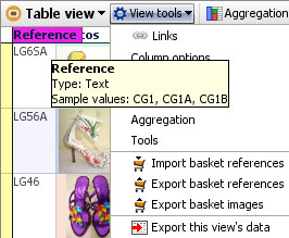
References are the values in a field (column) that are unique, that is, there is only one reference value for each record (row). (You should always test for duplicate references using the Table View Tools Tools > Select duplicate values option )
Import basket references- if you or someone else using data with the same unique identifiers have previously saved a reference list as the single column of values in a .TXT file, you can re-create the contents of the BASKET in your current Omniscope session using this command to import the external .TXT reference file. Omniscope will move all matching records (rows) into the BASKET universe automatically, and tell you if any references in the external file could not be matched.
Export basket references- typically, you use Side Bar filtering and power queries (together with geographic and image-based selection) to identify a sub-set of records on interest, and accumulate them in the BASKET universe. Before you exit, if you want to save (to share or re-use/re-create) the contents of the BASKET, you must use this command to export a .TXT file containing a list of the references currently in the BASKET.
Export basket images- Omniscope can be used to manage and select images grouped in folders (image sets) for web-sites, DataPlayers, and other uses. At any time, a selection of images in the BASKET can be exported as a new image folder using this command.
Export this view's data- used to export the entire contents of the BASKET universe in various file formats ( .IOK/.IOM, .XLS, .CSV, .TSV, .XML, etc.) using the Export Data wizard [544].
You can enable your users to browse the contents of the BASKET in any view(s), but given that they will have already selected these records and placed them in the basket for closer review, a free-floating instance of the Details View with the records navigation slider revealed can be the most effective.
To create a free-floating view, use ![]() Add View command on the Main Toolbar with the Open new window option ticked. From the Details View Toolbar, choose Show navigation controls to display the arrows and slider navigation at the top, and untick the Sync option, since this view is for user review of the BASKET universe only. Add a title, use the Links option to add buttons for the action links at the bottom, then hide the View Toolbar and users will be able to interact with their baskets record-by-record using a floating window something like this:
Add View command on the Main Toolbar with the Open new window option ticked. From the Details View Toolbar, choose Show navigation controls to display the arrows and slider navigation at the top, and untick the Sync option, since this view is for user review of the BASKET universe only. Add a title, use the Links option to add buttons for the action links at the bottom, then hide the View Toolbar and users will be able to interact with their baskets record-by-record using a floating window something like this:
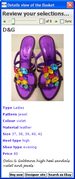
Omniscope allows you or your user to define a subset of Selected rows at any time, and from any view, usually just by using your mouse.
{update to version 2.5 in progress...}
The sidebars are used to display filter/query devices and other options on either the right or left-hand side (or both) depending on the tab-specific settings on the Main Toolbar: Toolbars options, which manage the display of the sidebars.
[2.5 Main Toolbar: Toolbars menu commands]
Whenever either Side Bar opens, there are three menus displayed at the top; the Devices drop-down menu, the Tools drop-down menu, and the right corner [X] to close the Side Bar. The first time the Side Bar opens, three configurable display options (Reports, Search All, and Exclusions) plus filter devices for all fields (columns) in the data set will be ticked and therefore visible on the Side Bar.
To configure or re-configure the Side Bar, click on the Devices drop-down menu on the upper left:

Except in a general 'Data Set' tab intended to show everything, you will probably not want filter devices for ALL the fields (columns) to be displayed on most pages. Some field values may not be relevant to the message or useful for selecting/filtering the displays on a given page. Use the Devices drop-down menu to untick those fields to hide their filter devices. Use the drag hands at the right to move filter devices up-wards or down-wards to achieve the desired display on the Sidebar. You can also move the filter devices themselves into a new order by dragging and dropping them with the mouse up-wards or down-wards on the Sidebar.
The three configuration options at the top of the Devices list (Reports, Search All and Exclusions ) will be displayed on the Sidebar only if you leave them ticked. Otherwise, untick these boxes and Report Page tabs will display across the top of the Main Toolbar (the default), Exclusions (Move and Keep with history) will show on the Main Toolbar (without history), and Search All will be available in the Portal View [12], when open.
Note: Side Bar settings are specific to each Reports Page, and must be changed page-by-page inside Reports Mode. Side Bar settings established outside Reports Mode (always hit Escape to make sure you are not working in a specific Report tab) will apply outside Reports Mode. If you create one or more Report Pages, you can either keep your existing Side Bar settings the same or change them to suit each Report Page. More on creating Report Pages. [435]
If you leave all three display configuration options ticked, the top of your Sidebar will look something like this:

Displaying Exclusions on the Sidebar has the advantage that you can expand the Exclusions device and monitor the history of your Moves and Keeps (see image below). This is especially useful when you are recording a power query sequence of ![]() Moves and
Moves and ![]() Keeps to send to someone else as a query file for use with their copy of the file (see below for more on query files).
Keeps to send to someone else as a query file for use with their copy of the file (see below for more on query files).
Displaying Reports on the Sidebar is useful when there are very few, or when there are many Report Pages that need to be arranged in groupings.
Like Search All above, any Sidebar text filter can be expanded to reveal a virtual keyboard for text search entry, with ANY and ALL multi-term search options. Omniscope text search works like a search engine, on one, several or all fields (columns)simultaneously. In any text filter, if you enter a single text string with no spaces, Omniscope will perform a prefix match, highlighting all records with text beginning with the search string. If you enter two text strings separated by a space and do not enclose them in "double quotes", you can search a field (column) of the data file for either one or both of the strings using the ANY or ALL search options. You can expand your search criteria to include values in other columns by simultaneously entering text strings in more that one filter device. To the right of each device you will see the hits in that column and at the top, in the barometer will show the combined record count.
Notice that whenever a query device is actively filtering the data set, the device panel colour turns orange:

Closing the Sidebar with filters set will prompt a message either to reset all the filters, or to convert the query settings to Exclusions. If you wish to keep the same record set in the IN Universe with the Side Bar closed, you must choose Convert to Exclusions, which means that the filter settings will be translated to the equivalent ![]() Moves and
Moves and ![]() Keeps that you can manage directly in the open views without the Sidebar.
Keeps that you can manage directly in the open views without the Sidebar.
The Sidebar Tools drop down menu displays commands that affect the data and/or all other Sidebar query devices. The first three of these are especially useful when managing the creation of Report Pages and using them in live presentations.
 | Reset variables- Variables are input values not contained in a column of the data set that you can include in formula fields to facilitate dynamic modelling and sensitivity analysis. When you specify a Variable, you define a minimum, maximum and a default value in the range. Each variable defined in a file can display a Sidebar slider enabling users to change the assumed value. Clicking on Reset variables returns all variables to their default values. For more on defining and using variables, see Formulas & Variables [476]. |
Reset configuration (views & layout) - returns the current view to a 'pristine' state, with all views closed and the Sidebar reset to opening default settings. Usually used to recover from confusing combinations of views and layout when constructing Report Pages.
Clear colour-by - each device has a small colour-by icon in the upper left. Clicking the device icon imposes the colouring scheme for that field (column) on all the open views that use colouring, like the Table View, the Tree View, etc. This command removes all overriding colouring schemes that have been set in the Sidebar (but not those already specified in the individual View Toolbars)
Halo function: Also include records with the same value in: - a powerful feature for managing groupings or clusters within a data set. Setting the Halo function changes filtering behaviour to include/maintain all records sharing a common value in the specified field (column). For more information, see Using the Halo function. [545]
[546]Expand all - expands all visible Side Bar devices
Collapse all - returns all Side Bar devices to their collapsed state (default on opening)
Add new variable - brings up the Add Variable wizard...see Formulas & Variables [476]
Edit variables - brings up the Edit Variable wizard...see Formulas & Variables [476]
Convert all to exclusions - Converts the current settings of all query/filter devices into Exclusions (the results of Moves and Keeps), thereby setting the green IN universe independently of Side Bar settings...allows Side Bar devices to be reset and/or hidden without changing the current composition of the data universes.
Import XML query file - XML query files exported from Omniscope by one user, say a business user identifying data quality issues with specific records (e.g. corrections or suspicious data) can be imported by another Omniscope user, say the Database Administrator, who wants to view just the records at issue and decide whether to parse the XML file to import the corrections into the source database.
Export XML query file - Exports the current query settings as an XML text file which other Omniscope users can open to recreate the same display, assuming they have the same .IOK file version open.
Right-clicking on any device displays a series of options for resetting/hiding the device, and changing the filter type. Changing the filter type is sometimes necessary to facilitate user interaction. In the example shown below, the field 'Node' is an integer number field, displaying as a range slider (the default) and with the 'Include empty (null) values' box ticked. If it was better to have users search for a specific number by typing it in, we could change the filter type to Text search...without changing the data type to Text.

Below the Filter Type command are a series of commands for managing each field. These commands are the same as those accessible from the Main Toolbar: Data > Manage Fields menu, and are discussed here [31].
Each text filter device has a drop down options menu that allows you to further refine the status and behaviour of the device.
Choosing the Show Text tools option provides more options.
The leftmost drop-down allows you to specify the text filtering options to be applied in this filter:
Substring (default) -
Word prefix -
Exact -
Regular Expression -
Applies to version 2.4 only
The Sidebars are used to display filter/query devices and other options on either the right or left-hand side (or both) depending on the tab-specific settings on the Main Toolbar Controls drop-down menu:
![]()
Whenever either Sidebar opens, there are three menus displayed at the top; the Devices drop-down menu, the Tools drop-down menu, and the right corner [X] to close the Sidebar. The first time the Sidebar opens, three configurable display options (Reports, Search All, and Exclusions) plus filter devices for all fields (columns) in the data set will be ticked and therefore visible on the Sidebar.
To configure or re-configure the Sidebar, click on the Devices drop-down menu on the upper left:
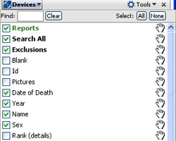 | Except in a general 'Data Set' tab intended to show everything, you will probably not want filter devices for ALL the fields (columns) to be displayed on most pages. Some field values may not be relevant to the message or useful for selecting/filtering the displays on a given page. Use the Devices drop-down menu to untick those fields to hide their filter devices. Use the drag hands at the right to move filter devices upwards or downwards to achieve the desired display on the Sidebar. You can also move the filter devices themselves into a new order by dragging and dropping them with the mouse up-wards or down-wards on the Sidebar. |
The three configuration options at the top of the Devices list (Reports, Search All and Exclusions ) will be displayed on the Sidebar only if you leave them ticked. Otherwise, untick these boxes and Reports tabs will display across the top of the Main Toolbar (the default), Exclusions (Moves and Keeps with history) will show on the Main Toolbar (without history), and Search All will be available in the Portal View [12], when open.
Note: Sidebar settings are specific to each Reports Page, and must be changed page-by-page inside Reports Mode. Sidebar settings established outside Reports Mode (always hit Escape to make sure you are not working in a specific Report tab) will apply outside Reports Mode. If you create one or more Report Pages, you can either keep your existing Sidebar settings the same or change them to suit each Report tab.
If you leave all three display configuration options ticked, the top of your Sidebar will look something like this:
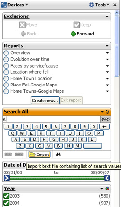 | Displaying Exclusions on the Sidebar has the advantage that you can expand the Exclusions device and monitor the history of your Moves and Keeps (see image below). This is especially useful when you are recording a power query sequence of Moves and Keeps to send to someone else as a query file for use with their copy of the file (see below for more on query files). Displaying Reports on the Sidebar is useful when there are very few, or when there are many Report Pages that need to be arranged in groupings. Like Search All above, any Sidebar text filter can be expanded to reveal a virtual keyboard for text search entry, with ANY and ALL multi-term search options. Omniscope text search works like a search engine, on one, several or all fields (columns)simultaneously. In any text filter, if you enter a single text string with no spaces, Omniscope will perform a prefix match, highlighting all records with text beginning with the search string. If you enter two text strings separated by a space and do not enclose them in "double quotes", you can search a field (column) of the data file for either one or both of the strings using the ANY or ALL search options. You can expand your search criteria to include values in other columns by simultaneously entering text strings in more that one filter device. To the right of each device you will see the hits in that column and at the top, in the barometer will show the combined record count. |
Note: Omniscope does not yet support an EXACT match option, so searching for numbers and text can return records whose values are supersets of the search term, i.e. a search for '22 ' will also display 222, 223, etc. leaving you to select the final records manually. (support for EXACT was added in version 2.5)
Notice that whenever a query device is actively filtering the data set, the device panel colour turns orange:
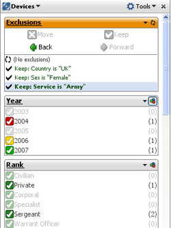 | Closing the Sidebar with filters set will prompt a message either to reset all the filters, or to convert the query settings to Exclusions. If you wish to keep the same record set in the IN Universe with the Sidebar closed, you must choose Convert to Exclusions, which means that the filter settings will be translated to the equivalent Moves and Keeps that you can manage directly in the open views without the Sidebar. |
The Sidebar Tools drop down menu displays commands that affect the data and/or all other Sidebar query devices. The first three of these are especially useful when managing the creation of Report Pages and using them in live presentations.
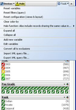 | Reset variables- Variables are input values not contained in a column of the data set that you can include in formula fields to facilitate dynamic modelling and sensitivity analysis. When you specify a Variable, you define a minimum, maximum and a default value in the range. Each variable defined in a file can display a Sidebar slider enabling users to change the assumed value. Clicking on Reset variables returns all variables to their default values. For more on defining and using variables, see Formulas & Variables [476]. Clear colour-by - each device has a small colour-by icon in the upper left. Clicking the device icon imposes the colouring scheme for that field (column) on all the open views that use colouring, like the Table View, the Tree View, etc. This command removes all overriding colouring schemes that have been set in the Sidebar (but not those already specified in the individual View Toolbars) Halo function: Also include records with the same value in: - a powerful feature for managing groupings or clusters within a data set. Setting the Halo function changes filtering behaviour to include/maintain all records sharing a common value in the specified field (column). For more information, see Using the Halo function. [545] |
Expand all - expands all visible Side Bar devices
Collapse all - returns all Side Bar devices to their collapsed state (default on opening)
Add new variable - brings up the Add Variable wizard...see Formulas & Variables [476]
Edit variables - brings up the Edit Variable wizard...see Formulas & Variables [476]
Convert all to exclusions - Converts the current settings of all query/filter devices into Exclusions (the results of Moves and Keeps), thereby setting the IN universe independently of Sidebar settings...allows Sidebar devices to be reset and/or hidden without changing the current composition of the data subsets.
Import XML query file - XML query files exported from Omniscope by one user, say a business user identifying data quality issues with specific records (e.g. corrections or suspicious data) can be imported by another Omniscope user, say the Database Administrator, who wants to view just the records at issue and decide whether to parse the XML file to import the corrections into the source database.
Export XML query file - Exports the current query settings as an XML text file which other Omniscope users can open to recreate the same display, assuming they have the same .IOK file version open.
Right-clicking on any device displays a series of options for resetting/hiding the device, and changing the filter type. Changing the filter type is sometimes necessary to facilitate user interaction. In the example shown below, the field 'Node' is an integer number field, displaying as a range slider (the default) and with the 'Include empty (null) values' box ticked. If it was better to have users search for a specific number by typing it in, we could change the filter type to Text search...without changing the data type to Text.
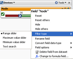
Below the Filter Type command are a series of commands for changing the filter types for each field. These commands are the same as those accessible from the Main Toolbar: Edit > Manage Fields menu, and are discussed here [31].
By default, Omniscope works with 4 defined sets/subsets of the integrated data set; ALL data, filtered IN data, filtered OUT data and Selected data. Files open with all records in the inegrated data set visible in the default filtered IN subset.
Omniscope has two query modes; Sidebar instant filtering, or Main Toolbar Selection, Moves & Keeps, whereby some records are transfered to the filtered OUT data subset as shown in the barometer.
You can define additional subsets of data which can be displayed alone or in conjunction with the defined data sets/subsets using Named Queries.
The Named Queries drop-down menu is immediately right of the Barometer, and provides all the commands required to define and manage Named Queries, combinations of filter settings or record selections which define selected or filtered subsets of the file data expected to be used frequently in configuring the views in the file. In the example below, 3 Named Queries have been defined; 'Basket One', 'Errors for Correction' and 'Other Named Query'. At right, the example Venn View toolbar has been set to display the records contained in the Named Query 'Basket One'.
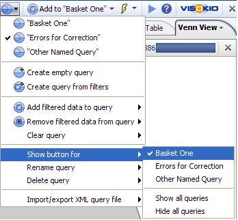 | Each View Toolbar includes a Data Subset drop down where you specify which of your defined Named Queries (in brown) should be displayed in the view:
|
Named Queries can be defined using either Create empty query or Create query from filters.
Create empty query - give the query you plan to populate a unique name for this file. The new query will appear at the top of the Named Queries drop-down list, and become a side menu option for commands such as such as Clear, Rename and Delete Query. The Show button for option places a button with the name of the selected Named Query/data subset on the Main Toolbar to the right of the Named Queries drop-down menu. These button(s) make it easier to manage adding or deleting selected/filtered IN records from multiple Named Queries. Once an empty query has been created, e.g. 'Basket One' or 'Errors for Correction' you can add filtered IN or Selected records to these queries at any time using Add or Remove selected/filtered data to query (if records are Selected, these records will be added/removed, if not, then the current contents of the Filtered IN subset will be added/removed to/from the Named Query you select from the sub-menu at right.
Create query from filters - this option lets you preserve the current pattern of filters set in the Side Bar as a Named Query. You can subsequently refine the data set defined using Add or Remove selected/filtered data to query.
Import/export XML query file- the definition of any query in the file can be saved in XML file format and exchanged with others using the same Omniscope file. This is useful for example, for highlighting anomalies and errors in the data requiring correction.
From version 2.5, most Omniscope View Toolbars include an Aggregation drop-down dialog which enables you to define an aggregated transformation of the underlying granular data set, and also define the aggregation functions to be applied across the aggregated values in each field (column). Each view on any given tab can use a different aggregated view as defined by the settings on the View Toolbar Aggregation drop-down.
Note: Formula columns can be set to apply the defined logic to the aggregated, rather than individual, row values by choosing 'Apply formula' as the aggregation function for the formula field.
Consider the unaggregated data set illustrated below and downloadable here [548]. Potential 'Aggregation Field 1' has 7 unique values, and potential 'Aggregation Field 2' has an additional 4 values uncorrelated with the 7 values in 'Aggregation Field 1'. In addition, there are Category, Numeric and Time & Date fields in the data set:
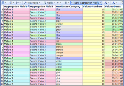 | 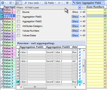 |
Use the Aggregation drop down menu found on most View Toolbars to define view-specific aggregated transformations of the underlying data set. The example above shows how to customise the drop-down fields and use the Preview window. In this case, the uniform value field 'Source' is being hidden, since aggregating by a single value will collapse the entire data set into one row. Notice that selections in the view are shown with brushing (fading) in the Preview window, enabling us to confirm that Value 1 is associated with both Second Value 1 and 2.
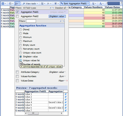 | Ticking a field on the Aggregation drop-down tells Omniscope to aggregate by the unique values in the chosen field, apply the default aggregation function to the values in the other fields, and display a view-level mini-barometer upper right with the aggregated record count. In this case, the result is 7 aggregated rows, one for each of the unique values, with the 'Values-Numbers' summed and the average (mean) of the 7 aggregated 'Values-Dates' displayed, since those are the default aggregation functions. Notice that the row headers now display how many individual records (rows) have been aggregated into each aggregated row. Aggregation functions are applied according to the defaults, but these can be changed for each field (or set to None) using the drop-down menus at right. Hover your mouse over each possible aggregation function (the list will depend on the data typing assigned to each field) and the tooltip will provide a definition of the function to be applied to that filed when aggregated. You can also change the default for a given field. |
Aggregating by multiple fields will usually increase the resulting row count, since all unique combinations of field values from all fields will become aggregate rows. IN the example below, the data set is being aggregated by both Field 1 and Field 2, resulting in 12 rows as shown in the mini-barometer:
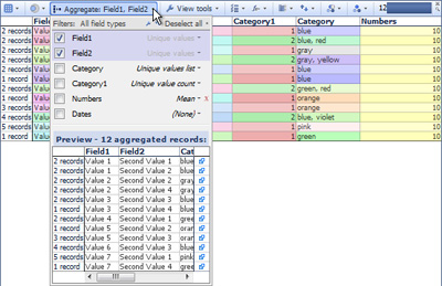 | In this case, the Category column was duplicated and two different aggregation functions applied; unique value count (which counts how many different colours are in each aggregated row), and unique values list (which lists all the unique values in the underlying rows). The aggregation function for 'Numbers was changed to Mean (average), which shows the original value of 10, which will stay the same no matter how many rows are aggregated, since the value was constant in the unaggregated data. The aggregation function for Dates has been set to None, which results in the Dates filed being hidden in the aggregated view. |
Many Views include an Aggregation drop-down menu, used to define aggregated views of the data, together with the function to be applied when aggregating each field (column). Aggregation differs from the presentational Grouping options available only in the Table View. Unlike Grouping, the end user is not meant to 'unroll' or 'drill down' defined aggregations to lower levels of granularity. User-interactive Grouping can be used in the Table View in addition to Aggregation. For example, a file with each row defined as an observation for a given day can be aggregated by week, then grouped by month and year. In the resulting presentational Table View, an end user would be able to unroll the groupings down to weeks, but to see the maximum granularity daily data, they would either have to remove the Aggregation settings (which they cannot do in a free Viewer) or just click to the 'Data Set tab (which they can do in a free Viewer).
The experience of the users of your files can be augmented in many ways using Omniscope.
Throughout Omniscope, there are many drop-down menus enabling the file publisher to manage the visibility of fields (columns) in user-selectable lists. Beginning with version 2.5, the field selection drop-down menus have been standardised and improved to help you find, choose and show/hide less useful fields (columns) to improve performance and prevent users from seeing inappropriate or uninformative fields as options on View/Device drop-downs.
You will find the improved field selection and management drop-down menus in several places:
This page describes:
For help with the drop-downs specific to a given View Toolbar, consult the Views Reference [21] for the relevant view.
The Colour button is the only data drop-down on the Main Toolbar. It allows you to pick a field from all the fields in your file, and then applies application-wide data colouring to all views with that capability. To revert, select "None" which will remove the application-wide colouring setting. [link to Data colouring]
In progress...
Tooltips allow you to display field values for records whenever your mouse hovers over parts of views. They appear as an extra floating display on top of views. For example, when you hover over a marker in the Graph view, or when you hover over a row header in the Table view.
You use tooltips when you want to be able to find out more information than is showing without having to click, when you don't want to clutter the display with this information up-front.
If the user hovers over a visual element that represents more than one record, although not a large number of records, they will see a multi-record tooltip, as shown below:

Tooltips are an extremely useful way to help users understand the key attributes of any record just by pointing with the mouse. However, you should be very selective, since trying to display too many fields in the Tooltips pop-up results in large, cluttered displays that obscure other important aspects of your display tabs.
By default, no fields are selected for tooltips. To pick the fields you want to display, use Settings > Tooltips > Fields (version 2.5+) or (Tools > Tooltips > Fields (verson 2.4) and tick fields, or drag to re-order.
If you have a file with image sets [414] configured, you can also pick an image to show in the tooltip. Use Settings > Tooltips > Image (2.5+) or Tools > Tooltips > Image (2.4).
{update to 2.5 in progress}
Omniscope can be used to align a set of images in a folder with records (rows) relating to each image, such that the images associated with each record (row) can be displayed in various views:
Before you can display images, however, you must associate one or more folders of images with the .IOK file as named image sets. Preparation for this involves saving a set of images in a single folder with a consistent naming convention that matches the text values in one of the columns of your .IOK file (it may be a column included just to hold the names of the images).
To save you having to find a lot of pictures in order to try this, the example below will use an Omniscope embedded demo file 'Works of Van Gogh', and its associated high-resolution image set. To take this tutorial, first click on the link below to download a zipped folder containing the images for the "Works of Van Gogh" demo.
Van Gogh Demo Image Set [549]105.3 MB (about 4-5 minutes on broadband)
Note: this folder contains many high-resolution images, making the download quite large. In order to bundle the entire folder of images together, this is a .ZIP file; do not click 'Open', click 'Save'. Download and unzip the folder, and save the unzipped folder on your desktop. Once you have saved the unzipped folder of images, open Omniscope and click Files > Demo files and select 'Works of Van Gogh'.
The embedded version of the demo file does not have the associated image embedded in it. Go to Settings > Images and you will see there are two options for retrieving the images, an automated, online service, and the manual approach. For this tutorial, to gain experience using the Add Images wizard we will try adding the downloaded image set manually. Select Add more images.
The Add Images Wizard will launch:
 | 1. Select Folder of images-Browse to the folder on your desktop containing the images and click select folder. 2. Choose field/column containing image references (the names of the image files)...in the Van Gogh demo this column is called 'Final Ref'. Select 'Final Ref' and you will see a sample image name displayed...in this case, a picture in the folder named J_30.jpg. 3. Choose format of references-Omniscope detects this automatically for demo files. 4. Select file extension to use...-this will show '.jpg' since all the images in the file already have this extension. 5. Give a unique name to this image set...change the suggestion from 'Images Set 2' to 'My Downloaded Images'. Check the example image at bottom right corner of the wizard and ensure that the correct image is displayed. Click OK to associate the named image set. |
To see your image set displayed, go to ![]() Add View on the Main Toolbar and add a Tile View. On the Tile View toolbar, click on the [ ? ] field (column) selector drop-down and select My Downloaded Images. You will see the images start to appear, but coloured. Go to the Colour selector to the right on the Tile View Toolbar and select 'none' to see the works coloured as van Gogh intended.
Add View on the Main Toolbar and add a Tile View. On the Tile View toolbar, click on the [ ? ] field (column) selector drop-down and select My Downloaded Images. You will see the images start to appear, but coloured. Go to the Colour selector to the right on the Tile View Toolbar and select 'none' to see the works coloured as van Gogh intended.
If you have an activated Edition of Omniscope (Professional or Enterprise) you can experiment with saving the file with your downloaded images embedded. At the same time, you can see the trade-offs between file size and image clarity/resolution that results when you reduce the image size to reduce the size of the .IOK file. To save a version of your file click File > Save as. The Export File dialog will appear:
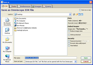 | Note the commands available along the right hand side: |
Tick the box 'Reduce Image size' . Give the new version of the file you are saving with embedded images a name, such as Works of Van Gogh 200x150.iok. Click Save and you will see an image reduction dialog that enables you to reduce the size of the images to reduce file size, but at some cost in terms of image clarity.
| Accepting the existing image sizes will result in a file of over 100 MB, so let's try reducing the dimensions of the pictures by 50%, to 200x150 (hence the name of the file we are saving). Change the maximum values to 200 wide and 150 high and click OK. Omniscope will save the file with reduced embedded images. The resulting file is about 14 MB, still large, but not bad for an entire art exhibition in a portable, searchable file! |
{update for 2.5} Open the new version of file and close all the open Views except the Tile View, which should be configured to display the now embedded image set My Downloaded Images. On the Tile View Toolbar, select the movie camera Slide show icon to the left of the Add to basket icon far right. Click 'Start slide show' and choose full screen sub-option. Look at the image quality on your screen. If it is acceptable for the audience/screen resolutions you intend, consider reducing the images more to reduce the .IOK file size further. If the image quality full screen is not acceptable, you may have to reduce the maximum size of the images less (increasing the file size), or configure the views such that images are never displayed so large. To do this, repeat the steps above, and set larger maximums in the 'Reduce image size' box.
Before you can display images related to your data set, you must first associate one or more image folders with your IOK file as named image sets. Preparation for this involves saving a set of images in a single folder with a consistent naming convention, such that one of the columns of your IOK file (it may be a column included just to hold the names of the images) contains the same text values as the file names of the images in the folder, i.e. 'picture1', 'picture2' etc. Any image naming convention can be used, so long as the same exact text strings are present in one of the columns of your data set. You can omit the file extension from the data column if all the images have the same extension, e.g JPG or GIF. If the images are mixed format, the names in the data column must include the file extension for at least one of the formats.
There are 3 ways to display images in Omniscope:
It is also possible for Omniscope to display multiple images per record, provided you have entered multiple values in the image reference cell by declaring the field (column) to be Tokenized (for more detail, see Tokenized data). [27] If you enter multiple image references per cell, the Tile View will show the first image by default, but you can change this in the Tile View View Tools > Advanced sub-menu. The Details View, pop-up windows and Slide shows will all display the tokenized images for each record.
The Tools > Images menu contains two options:
Add Image Set- launches the Add Image Set wizard documented below.
Modify Image Set (only visible if an image set is already associated with the file)- launches the Edit Image Set wizard, which is effectively the same as the Add image set wizard. The modify image set option is usually used to re-import or re-embed an image set using the Refresh embedded images button at the bottom. Warning: Only use this command if you are sure you know the location of a complete new image set, ideally containing images at the original resolution, so that you can remove the old one and replace it with a new one.
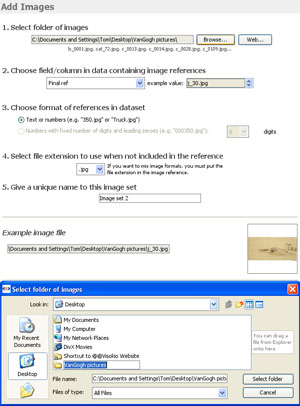 | 1. Select Folder of images- Browse to the folder containing the images. If the file is located on a remote machine accessible via the web, click Web and enter the web address of the folder. 2. Choose field/column containing image references- specify which field in your data file contains the names of the image files, and confirm by cycling through a range of example values. 3. Choose format of references- specify which format the image names are in 4. Select file extension to use- for image sets with mixed formats (e.g. .JPG and .GIF), you must include the file extensions for the non-default format as part of the image names in the reference field, but you do not need to add the extension to the default format references. 5. Give a unique name to this image set- give each image set you create a descriptive name. Check the example image at bottom right corner of the wizard and ensure that the correct image is displayed. Click OK to associate the named image set with the open IOK file. |
To see your image set displayed, go to ![]() Add View on the Main Toolbar and add a Tile View. On the Tile View Toolbar, click on the [ ? ] field (column) selector drop-down and select 'My Image Set' or whatever unique name you have used. The Tile View should display all the images in the image set. Missing images will be substituted with a red tile, but you can create a special image to substitute the missing ones, give it a name, add it to the images folder, and add its name to the empty cells in the image reference column.
Add View on the Main Toolbar and add a Tile View. On the Tile View Toolbar, click on the [ ? ] field (column) selector drop-down and select 'My Image Set' or whatever unique name you have used. The Tile View should display all the images in the image set. Missing images will be substituted with a red tile, but you can create a special image to substitute the missing ones, give it a name, add it to the images folder, and add its name to the empty cells in the image reference column.
Once you have associated and image set, you can save the IOK file with your images embedded. You can also experiment with the trade-offs between file size and image clarity/resolution when you reduce the image sizes to reduce the size of the IOK file. To save a version of your file click File > Save as IOK. The File Save wizard will appear:
 | Note the commands available along the right hand side: |
If you embed large numbers of large images without reducing their size, the resulting IOK file can become far too big. In general, images can be substantially reduced from their original size without affecting the quality of the display on computer monitors. To test the effects of reducing the image file sizes, tick Reduce Image size. Give the new version of the file you are saving with reduced embedded images a name, such as 'My File with max picture size 200x150.iok'.
| Click Save and you will see an image reduction dialog that enables you to reduce the maximum dimensions of the images, thereby reducing the size of the IOK file, but sometimes at some cost in terms of image clarity. If you set maximum values for width and height, Omniscope will scale down any images with dimensions exceeding the maximum until the relevant dimension is within the maximum.
|
The size of the images displayed is not affected as much as the resolution, since Omniscope manages the sizing of the images dynamically within each display.
Open the new version of the file and close all the open views except the Tile View, which should be configured to display the now embedded image set My Downloaded Images. On the Tile View Toolbar, select the movie camera Slide show icon to the left of the Add to basket icon far right. Click Start slide show and choose full screen sub-option. Look at the image quality on your screen. If it is acceptable for the audience/screen resolutions you intend, consider reducing the images more to reduce the IOK file size further. If the image quality full screen is not acceptable, you may have to reduce the maximum size of the images less (increasing the file size), or configure the views such that images are never displayed so large. To do this, repeat the steps above, and set larger maximums in the Reduce image size dialog.
You can use Omniscope to manage large collections of images and other media by using your hard disk as a data source.
Visit File > Open image collection [412] or File > Open folder of files [411] to get started.
{update to version 2.5 in progress}
Links extend your file users' experience to include content not contained in the Omniscope .IOK file itself. By adding links, anyone can integrate other related content (documents, images, web pages, audio-video clips, etc.) into their .IOK files via their local network, and the open web. You can include full links in a column in your data, or specify data-driven (parametric) links that Omniscope composes on the fly, combining pre-defined strings with user-selected values in cells to create valid URLs.
Omniscope comes with a number of preconfigured links to free web services, such as a Google search, Wikipedia reference or Yahoo stock price charts. Once created, links can be attached to any field using the Links command available in many View Tools menus. Any number of Web Views [540] can be configured to display the results of selected links, or the users' default browser is used.
From the Main Toolbar, the Tools > Links menu enables you specify links and make them available for use within your .IOK file using the Add web link, Add local link and Preconfigured links dialogs:

The Add local link, Add web link and Preconfigured links dialogs are simple to use and allow anyone to create dynamic local and web links combining text strings typed in just once (like a network file server/folder locations or web site domain names) with the values of fields contained in the .IOK file. The result is user-selected, dynamic, data-driven links that extend users' access to related information dramatically.
File folders located on your machine (or on other machines accessible to you over your local networks) can contain documents, images, audio and video clips, practically any kind of digital content related to your data. For example, you may store a folder of documents on a remote file server that users of your .IOK file may wish to consult. If you have a reference name/number for each document (or the enclosing folder for groups of documents), including the references as a column in your .IOK file will permit users of your file to link to the folder or specific documents, audio or video clips, etc. inside.

Using the Add local link wizard, you build up the link by:
1.) Browsing to the network location containing the files you are linking to,
2.) Building the file name by adding in any text that does not change (e.g. 'fileserver' in the example above) and specifying each of the fields in your .IOK file containing values that will add specificity to the location/document/file the user will be linking to. To delete, backspace and try again. Once have have fully specified the link to an existing file/document,
3.) Try the link across a number of different records ( in the example above, there was no document found)
4.) Name the link once you are sure that the link is correctly specified and working across the full range of records
Once the link is fully configured, it will appear with the name you have given it on all menus relating to links in the file. If you then assign the link to a field (column) in the data set, you can create an underlined link from all the values in that field that launches the link whenever the user clicks on a value in that field (column). You can assign a link to a field in several ways, the simplest being to open the Table View, then click View tools > Links and select the field from the list that appears. In the Table View, the values for that field (column) should become underlined once you assign the link. You can also display local links as action buttons/links in Details Views and pop-up windows.
Note: You can assign a link to any field (column), not just the fields whose values comprise part of the definition of the link. For example, you could define a link made up of the reference numbers of documents and some other text, but assign this link to the column containing the title of the document. Clicking on the title would launch the document, using the reference number from that record, (not the title) as an argument to complete the definition of the link.
Any resource available on the open web can be linked to an Omniscope .IOK file using the Add web link wizard.

The Add web link wizard process is similar to building local links. Use the drop-down to specify the web protocol for the resource (usually http://) then type in the part of the URL/web address that is not contained in one of the fields in you data set. Next, select one or more fields from your data set, typing in any necessary separators like /, %20, etc. between the inserted fields. To delete mistakes, backspace and try again.
Once you have configured a valid URL/web address, test the link by cycling through various record field values, and clicking on the displayed link. Once you are sure that it is working as you expect, give the link a name. The link will now be added to the list of links available in your file. In the same way as local links, you can associate web links with any field (column) and they can appear as action buttons/links in Details View and pop-up windows. Web links can also be associated with Web Views by selecting the links from the list in the Web View Toolbar drop-down. For more information, see Using the Web View. [540]
Omniscope contains a menu of preconfigured links to many free, popular web services you can add to your files for the convenience of file users.
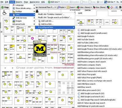
Free web services tend to expect a single cell value, such as a search term/string of text, a recognised identifying number like a stock ticker, CUSIP or ISIN (securities) or an ISBN number (books). If your data set includes fields (columns) that can be submitted to these or other web services (see Adding Web Services [550]), you should consider configuring these links in your files. You can set the results to display in one or more Omniscope Web Views [540], or the user's default browser.
{update to version 2.5 in progress}
Links extend your file users' experience to include content not contained within the Omniscope IOK file itself. By adding links, anyone can integrate related external content (documents, files and web pages) into their IOK files, with one-click access via their local network, and the open web.
Links in Omniscope allow you to link a single record to some related online content or service, optionally passing field values to the remote web server (in a single string), allowing you to reference content and even gather field values from external websites.
Note: If you need to post multiple records to a server, you need to use Settings > Web Services [17] instead.
You specify links and make them available for use within your IOK file using the Add web link, Add local link and Preconfigured links dialogs available from Settings > Links menu on the Main Toolbar.
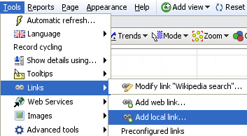
The Add local link, Add web link and Preconfigured links dialogs are simple to use and allow anyone to create dynamic local and web links combining text strings typed in just once (like a network file server/folder locations or web site domain names) with the values of fields contained in the .IOK file. The result is user-selected, dynamic, data-driven links that extend users' access to information dramatically.
File folders located on your machine (or on other machines accessible to you over your networks) can contain documents, images, audio and video clips, practically any kind of digital content related to your data. For example, you may store a folder of documents on a remote file server that users of your .IOK file may wish to consult. If you have a reference name for each document (or the enclosing folder for groups of documents), including this information as a column in your .IOK file will permit users of your file to link to the folder or specific documents, audio or video clips, etc. inside.
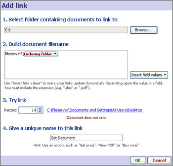
Using the Add local link wizard, you build up the link by:
1.) Browsing to the network location containing the files you are linking to,
2.) Building the file name by adding in any text that does not change (e.g. 'fileserver' in the example above) and specifying each of the fields in your .IOK file containing values that will add specificity to the location/document/file the user will be linking to. To delete, backspace and try again. Once have have fully specified the link to an existing file/document,
3.) Try the link across a number of different records ( in the example above, there was no document found)
4.) Name the link once you are sure that the link is correctly specified and working across the full range of records
Once the link is fully configured, it will appear with the name you have given it on all menus relating to links in the file. If you then assign the link to a field (column) in the data set, Omniscope will create an underlined link from all the values in that field that launches the link whenever the user clicks on a value in that field (column). You can associate local links with any field (column) and they can appear as action buttons/links in the Details View and pop-up displays.
For more information on how Omniscope builds links, please see Absolute and relative links [551].
There are many free reference and look-up services available on the web. Omniscope includes a library of preconfigured links you can use to extend the reach of the users of your file, eliminating the need for them to re-type what could be long and complex codes or foreign languages in order to access a service.
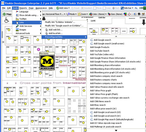
Free pages tend to expect a single string of text, i.e. a search term/string, a recognised identifying number like a stock ticker, CUSIP or ISIN (securities) or an ISBN number (books). If your data set includes fields (columns) that can be submitted to these or other web pages (see creating custom links below) you should consider configuring these links in your files You can specify that the results be displayed in one or more Omniscope Web Views [540] or the user's default browser.
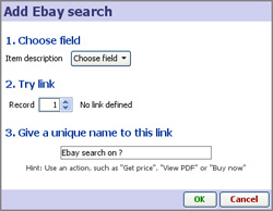
If you would like to offer other free preconfigured links to be added to the list included in Omniscope, or otherwise communicated to our users via our web site, please contact us [51].
Any resource available on the open web can be linked to an Omniscope IOK file using the Add web link dialog:
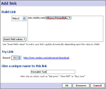
The Add web link wizard process is similar to building local links. Use the drop-down to specify the web protocol for the resource (usually http://) then type in the part of the URL/web address that is not contained in one of the fields in you data set. Next, select one or more fields from your data set, typing in any necessary separators like /, %20, etc. between the inserted fields. To delete, just backspace and try again.
Once you have configured a valid URL/web address, test the link by cycling through various record field values, and clicking on the displayed link. Once you are sure that it is working as you expect, give the link a name. The link will now be added to the list of links available in your file. In the same way as local links, you can associate web links with any field (column) and they can appear as action buttons/links in Details pop-ups and views. Web links can also be associated with Web Views by selecting the links from the list in the Web View > View Toolbar > Links drop-down. For more information, see Using the Web View. [540]
{update to version 2.5 in progress}
Omniscope is a universal web service 'hybrid' desktop/web client. Using the options available under Settings > Web Services, you can define standard web services in your IOK file, allowing your users to select some records and "post" them to a remote server which will process the request using the data, then present a results web page viewable in a Web View of the Omniscope file, or the users' default browser. A number of free web services are available preconfigured, or enter the details of a web service server yourself.
Note: Omniscope currently supports posts of values from a single column only. If you have a solution requiring multi-value, multi-column posts, please contact us [86].
Omniscope integrates with web services to offer a hybrid 'best of both worlds' combination of powerful desktop client/user interface with the ability to send user-selected or modified subsets of data (including user input data) back to remote servers for further processing. Corrections and updates can be sent back the the central data repository for refresh back into Omniscope, or remote server results can be immediately displayed using one or more Web Views [552] or the default browser on the users' machines.
Currently, Omniscope supports exporting to remote servers of any number of values (references) from a single field (column). Behind the scenes, Omniscope submits an POST to an HTTP server listing the record identifiers from a field of your choosing. You can define a formula field that collapses multiple user-changed fields into a single delimiter-separated column for posting back to the central data source. You can also write formulae files that return values read from remote web services. If you envisage a solution that requires posting a table of selected or modified values (more than one column) please contact us. [86]
Web services you want to make available from within each file are defined using the Main Toolbar Settings > Web Services dialog:
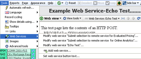
From the Main Toolbar, the Settings > Web Services menu offers the following options:
Modify Web Service- allows modification of all the parameters associated with any web service already configured in the file or remove the web service from the file. The parameters are the same as those shown below in the Add Web Service wizard: HTTP POST URL; Web Service name; ID field (the field (column) from which selected values should be exported) and the Record count limit, which sets the maximum on the number of values posted at a time.
Add Web Service- selecting the Add web service option opens the Web Service configuration wizard:
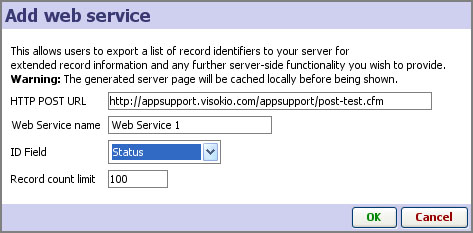
Add your own Web Service configuration to the file by supplying your own values for:
HTTP POST URL: the full URL of the server file/page responding to POSTs
Web Service name: Name you give that appears on the Omniscope Web Services menu. In the example above there are 3 names for 3 different services available from the file.
ID Field: the field (column) name in the Omniscope that contains the values to be exported to the Web service being configured. Can be different for each service
Record count limit: Can be any number of values, set to 100 by default
Omniscope includes a test web service that 'echos' whatever field (column) of values you choose to send. Try configuring this service using the URL given, with a name like Echo Test, and selecting a field in your data set. In one of the views in Omniscope, select less than 100 records, and in the Main Tool Bar, click on the 'Echo Test' web service. If you have not configured a Web View in Omniscope to display the results, the default browser will open and display the echo results. If you have configured a Web View to display the web service results, they will appear in that open Web View.
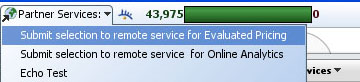
Set Web Service button text- Sets the display/hover value for the Web Services menu button...'Partner Services' in the example shown above.
For more discussion of options for building web-integrated data publishing solutions using Omniscope, consult our KnowledgeBase sections on Web Integration [553] and communicating with Web Services. [554]
Omniscope opens with a single default tab, but any number of tabs can be added as you evolve your file through various phases of the configuration checklist [384]. Any combination of views, settings, filters, titles and annotations can be saved on persistent Tabs displayed across the top of the Main Toolbar, or optionally on the Sidebar. Many settings are applied at tab level, and changes to tabs must be Committed using Main Toolbar: Tab > Commit changes before they become persistent.
If you close and save an Omniscope file displaying a given tab, this file will open next time displaying the same tab. Users of the file simply page through the tabs in order just as they would a presentation slide show. Using the Main Toolbar: Toolbars [445]command menu, additional navigation options can be displayed using Toolbars > Floating tab navigator or Next/previous buttons, to display either a faint, on-hover Reports Navigator in the lower left corner (that emulates PowerPoint), or forward and back screen arrows in the bottom corners, or both. The right and left keyboard arrow keys can also be used to page through the file when giving a live presentation for example.
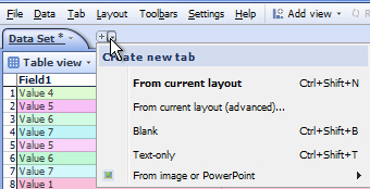 | Create new tab:
Text-only -
|
Note: For options covering aspects of the look and feel that apply to more then one tab, see the section on Reports & Presentations [430].
Sidebars are used to enable users to filter records (rows) quickly and easily. Sidebar settings are tab-specific, so you should configure the Sidebars on each tab to meet the needs of users on each individual tab.
{update to 2.5 in progress}
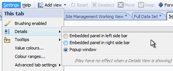 | Embedded panel in left sidebar -
Embedded panel in right sidebar -
Popup window - the default, floating display screen which can be re-sized.
|
As noted, on Tabs where the Details View [20]display is in use, some of these settings may have no effect to prevent redundent displays of information
Double-clicking on a Table View row hear will display the Details pop-up, with the configuration Details Toolbar displayed at the top by default. if you to not see athe configuration toolbar, check to see that the Main Toolbar: Toolbars > Details toolbar display option is ticked (the default setting for Working mode layout).
Applies to version 2.4 only
In addition to the Details View [20], Omniscope can display configurable record-level details as pop-up windows and embedded Sidebar panels. Open a Sidebars on your file and try each option for viewing details outside of the Details View.
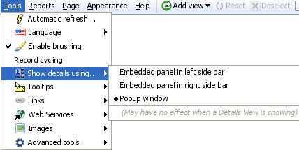
Hidden by default, the Cycling Toolbar is revealed at the bottom of the display from Main Toolbar: Toolbars > Cycling toolbar
![]()
![]()
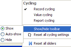
Applies only to version 2.4;
With the exception of the Table View, Omniscope views do not show the all the values associated with individual records (rows) or small groups of records. Once you have filtered down to a relatively small group of records of interest (using Selections followed by Moves and Keeps, instant Sidebar filter devices, or selecting a Named Query data subset) you have several highly-configurable options for viewing some or all of the details for one or a group of selected records.
If the Table View is open, and no Details View is open, selecting/double clicking on a row header (left-most part of a row) will display the details for that record- either as a separate pop-up window (the Details window) or as an embedded panel in the left or right Sidebar (you set this option from Main Toolbar: Tools > Show details using ).
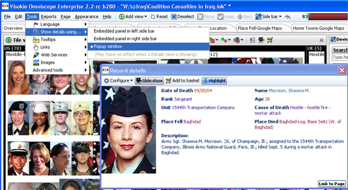
Whenever the Details View [20] is open, clicking on row headers or links set to display details will display inside the Details View. Only if the Details View is closed will the Details pop-up window or embedded panel options display. Whenever the Details View is open, the settings for that view (columns to show, etc.) will be used. When the Details View is closed, the settings for the pop-up Details Window or embedded Sidebar panel display will be used. Note that these settings are tab specific. If you wish to alter them in a given tab, you must open that page, make the changes and commit your changes to make them persistent.
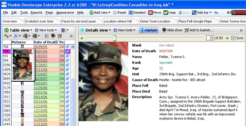
Every View Toolbar has a View Details icon next to the Add to Basket icon on the right hand side. This command opens a tabular view of either the selected records in the view, or all data in the view, showing the fields set to be visible in the Table View, even if the Table View is not visible. The View Details option is like opening a temporary Table View. Like the Table View, double clicking on the row header, or on any underlined link set to open the Details Window/Side Bar panel, will display individual details for that record. You are always at most 2 clicks away from full details on any record using the View Details option on any View Toolbar, followed by clicking on the row header or details link in the View Details pop-up window.
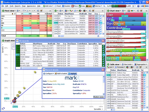
Warning: The fields (columns) displayed in the View Details pop-up table window are the same (and in the same order) as the settings governing the Table View. For an given tab, you must configure a Table View (even if the Table View is not normally open on the Reports Page), in order to control the order of the visible fields in the View Details pop-up for that tab. If you do not do this, the settings for the Table View at the time the tab was created will be used. If you later change the settings for your working display Table View, the changes will not automatically be made in other tabs unless you select Apply these changes to all Table Views and then explicitly elect to apply the same settings to all tabs, or else you return to each tab and change the Table View settings individually.
If Settings > This tab > Brushing enabled (the fading of unselected records) is not enabled, whenever a single record is selected, the position of that record is highlighted in aqua-blue in all open views., as shown above. Open Table Views will scroll to reveal the selected record. Use highlighting to see the positioning of a record in plots, such as the Graph and Chart Views, and read off values for various fields of the selected record in all open views. If you are using a colour-by setting on the Sidebar, highlighted rows will be partially highlighted, so that you can still discern the colour assigned to the highlighted record (row). You can turn this feature off by clearing the Highlight button on the view/pop-up toolbar.
Hovering on the Main Toolbar barometer reveals the control panel for record cycling. Record cycling automatically steps through the records in the universe you select and displays the position of each record in all open views using highlighting. If you have a Details View open, or details windows showing on the Side Bars, then the details for each record (including any related images) will be displayed as cycling steps through. Cycling is turned on, paused, stopped, fast-forwarded and fast-reversed using the green control icons under the barometer.
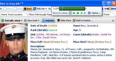
Clicking on the Options button displays the record cycling configuration panel. Options available include Loop, which plays the cycle continuously once started; Play on open, which starts cycling automatically when the file is opened; Universe: which selects the data universe from which the records will be cycled for display; and Record order which sets the field used to order/sort the records to be displayed.
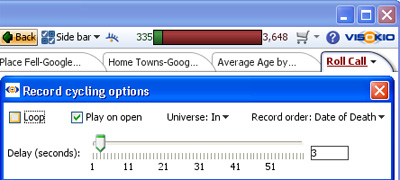
Warning: If you have global record cycling enabled, and you turn off the Highlighting option, the record cycling will stop. To re-start record cycling, hover your mouse on the barometer to expose the global automatic record cycling menu, and click on the green forward arrow to re-start.
Note: Version 2.4 has improved control of cycling options, see using the Cycling Toolbar [556]
Most View Toolbars feature a Slide show option. This option is used in files with associated or embedded image sets to display the image(s) associated with each record in a special Slide show display window. This window can be any size and can be displayed on another monitor. Unlike record cycling with the details view, slide shows can show multiple images associated with each record using tokenized file names in the picture column. For more information, see Tokenized data [27]
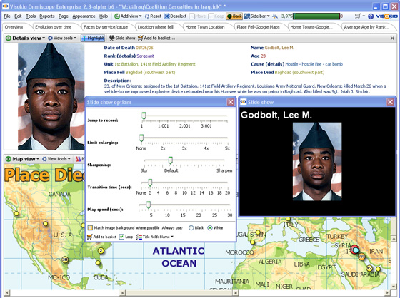
From the View Toolbar, click on the Slide show icon to reveal the configuration options panel. Options available on this panel include:
{update to 2.5 in progress}
Omniscope is not only for managing data, it is also for sharing data with others in a form that they can understand it fastest and make the best use of it.
There are three ways of adding your own text to your presentation:
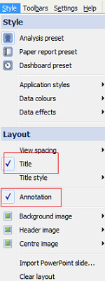 | To add a Title and Annotation to the Tab, the user can select the option “Style” from the main toolbar and then select “Title” or Annotation Option. To see how to edit Titles & Annotations visite T [557]ab-titles-annotations [557] . |
Displaying View Header & Footers
| The user can Add and Display a header & Footer, by selecting the option Tools>Toolbars styles>Header or Footer.
Those options are also available from the main menu under Toolbars. |
Footers are edited and styled using the Text Editor Menu bar [558]
Any number of Content Views can be added to each tab and sized the compliment the data-driven views. The Content View enables you to enter free text, incorporating dynamic formulae and links, images and other content to help make your report tabs come alive.
Free text entered in the Content View is edited and styled using the Text Editor Menu bar [558]
More on using the Content View [18]
You can import PowerPoint slides and create new Text Tabs from Tab > New.
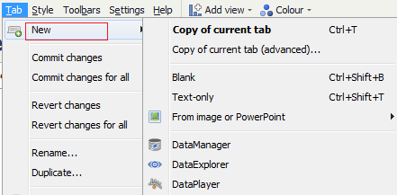
Images and PowerPoint slides arre not editable in Omniscope and are imported as is.
Free text entered directly int a Text Tab is edited and styled using the Text Editor Menu bar [558]
-----------------------------------------------------
Edit Annotation [559]
Web and File Link [560]
Formula [561]
Aggregate [562]
Subset: Filtered data [563]Aggregate [562]
Subset: Filtered data [563]
Like presentation packages, ach tab of an Omniscope file can be written as a presentation slidde, with top titles and bottom annotations.
Create a Title
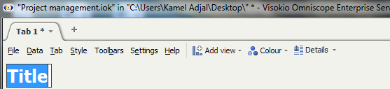 | To create a Title to the Tab, select “Style” from the main toolbar and then select “Title” A temporary name“Title” will automatically appear highlighted at the top of the screen. Type in the title you would like to give to your project and hit Enter. |
Back to the Top [564]
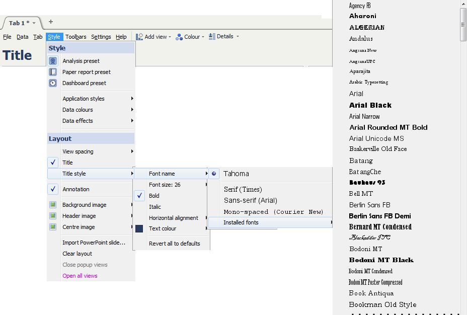 | Omniscope gives the user the option to change : Style,colour, size and alignment of the font.. All these options are available under Title style Back to the Top [564] |
 | The user can delete the title at any time. Select Style in the main toolbar and unselect the option “Title”. A pop up will appear with a warning message:
This will erase the title. Are you sure? - Press Ok to erase the title from your project.
-Press Cancel to keep the title in your project. Back to the Top [564] |
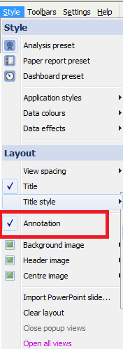 | Select “Style” from the main toolbar and select the Annotation option. A temporary name “Annotation” will automatically appear highlighted at the bottom of the screen. Type in the annotation notes you would like to add to your project and hit Enter. Back to the Top [564] |
To see how to edit /change the font/ insert image .... to the Edit box please click on this link: Text Editor [74].
 | This will erase the Annotation.Are you sure? - Press Ok to erase the title from your project. - Press Cancel to keep the title in your project. Back to the Top [564] |
Throughout Omniscope, wherever you have the option to add your own free-form text to the disply, the Text Editor Menu bar will display.
Click on Edit to edit the annotation.
![]()
Edit HTML Source
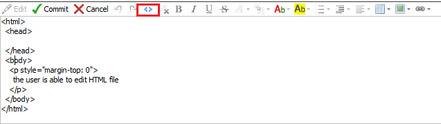
Remove formatting
Annotation allows the user to remove text formatting by selecting the text edited, and clicking ![]() button
button
This will turn the text back to the default setting.
The user is able to change the font of the text from Bold to Italic by using the button ![]() or
or ![]() .
.
Omniscope also allows the user to use key short cuts to turn the text to Bold (CRTL+B) or italic(CRTL+I).
The user can underline text by highlighting the text and selecting the button![]() or pressing (CRTL+U)
or pressing (CRTL+U)
The user can Strike through a text by highlighting the desired text selecting the button![]() or pressing (CRTL+G)
or pressing (CRTL+G)
The user can change the Font of the text by highlighting the desired text and clicking on ![]() .
.
The user can change the Font of the text by highlighting the desired text and clicking on ![]() .
.
The user can change the Text colour by highlighting the desired text and clicking on ![]()
The user can also highlight text by selecting the text and clicking on ![]() .
.
The user can insert bullets and numbers when selecting this button ![]() .
.
These options are available by clicking this Button ![]() .
.
A pop up appears asking to configure the table: number of row/column/Scale/table width/ Borders
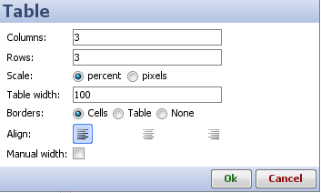
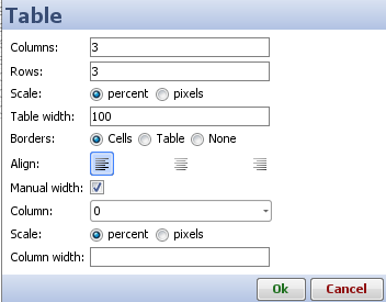
After a table has been created, the user can still modify its properties by selecting the table and pressing ![]() again, Options are:
again, Options are:
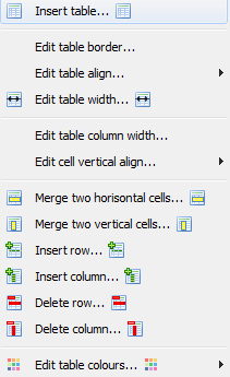
The user can enter an address (URL) to show a web based image:
All those options are available from Insert Image’s button
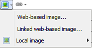
The user can link any web page or file into the annotation window
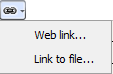
The Main Toolbar: Layout [25] menu groups most of the commands used to manage the elements of a tab outside of the views to be displayed on that tab.
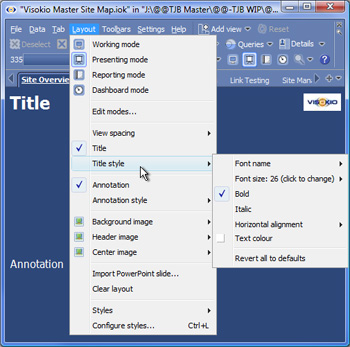 | Edit modes [433] - you can modify the default settings for layout modes and add you own to a given file.
|
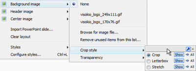 |
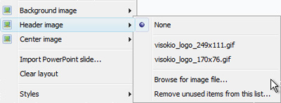 |
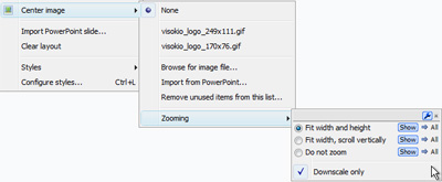 |
Import PowerPoint slide - you can import an existing PowerPoint slide into a tab
Clear layout - removes all the display elements outside of the views displayed on the current tab
Styles - combinations of settings that can be applied to a specific file, and also shared with other users. You can use standard pre-configured Styles, or create a custom organisational Style to apply to all Omniscope file created by a given organisation. For more information, see Styles & Configure styles [434]and also the KnowledgeBase section on sharing custom styles [565].
You can modify default Layout modes, and add your own Layout mode options to any given file. Layout modes can be applied to any or all the tabs in the file. You can show or hide Layout mode option icons on toolbars, and assign icons for exposing the options on the Main Toolbar. The Main Toolbar: Layout > Edit Modes... dialog is used to customise Layout modes:
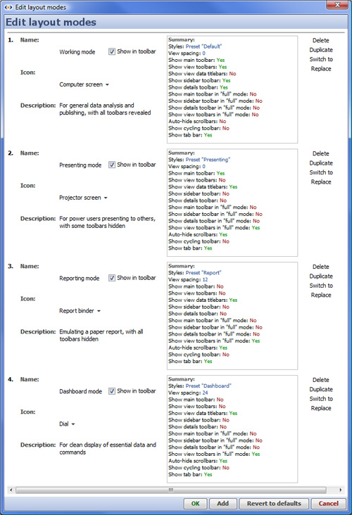 | Delete - deletes the corresponding Layout mode option from the current file. Duplicate - creates a new mode option below with the same settings as the existing Layout mode being duplicated. Active or Switch to - Active indicates which Layout mode settings are currently being displayed. If no options are showing Active, click Switch to next to the mode settings pane you wish to display, setting it to Active, then click OK. Replace - copies the currently active mode settings into the corresponding mode options pane [OK] - applies the selected settings and displays the Active Layout Mode [Add] - adds a new mode options settings pane at the bottom of the list [Revert to defaults] - returns all settings to their default values and deletes any additional Layout mode options you may have create [Cancel] - closed the dialog without saving any changes. |
Layout modes are not exportable for use in new files configured by others, and do not include the settings available when configuring Styles [434]. If you want to use a customised Layout mode option in a new file, delete the data from an existing file and change its source, thereby preserving the custom Layout. Options which can be changed to customise or define new layout modes are described below:
Styles -
View spacing -
Show main toolbar -
Show view toolbars -
Omniscope enables anyone to create a corporate Style corresponding to your corporate colours and presentation standards, using a combination of official logos, font settings, colours and effects defined using the Layout > Configure styles dialog. Change the settings and observe the result interactively. Once you are satisfied with all the settings, name and save your custom Style preset and it will be added to your Layout > Styles menu. You can also copy this customised style preset to others in your organisation, so that the official corporate style becomes available in the same menu to everyone configuring files (see below).
Default style |
Presenting style | |
Reporting style |
Dashboard style |
Each of the default Layout modes also has a default style is optimised for the different uses:
Working mode: for general data analysis and file configuration, with all toolbars revealed.
Presenting mode: for power users presenting to others interactively, with some toolbars hidden.
Reporting mode: for routine reports and printing a static copies, with all toolbars hidden.
Dashboard style: use this for clean, remote displays with frequently refreshing data.
You can edit the default layout modes [433]on a file-by-file basis, but you cannot share these settings with others configuring new files as you can using custom Styles.
Styles are combinations of display settings you can change using the Layout > Configure styles dialog. These settings control most of the visible aspects of each file, outside of the controls available within individual views. A pre-defined Style called 'Default' is used for every file unless you make a change. A menu of alternative pre-defined styles is available under Layout > Styles. You can apply different 'looks' by changing the style applied to the open file.
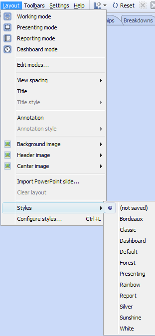 | 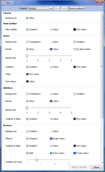 |
If you change any settings relative to the current style preset, the Preset selection drop down will show that the new altered preset is not saved. Click Save to give a name to the newly-modified style preset and save it to your installation, from which it will be available for future use, and transferable in the form of an .XML file you can copy across machines.
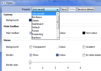 | The settings corresponding to the new style preset are saved in a local .XML file named {YourPresetName}.XML. Anyone who creates a new file from an existing file can use the same style preset, which is part of the file. However, anyone creating a new file will not have access to the custom corporate style unless it is first copied to their machine [565].
|
Relates to version 2.4 only; from version 2.5 Report pages are referred to as Tabs.
Any combination of views, settings, filters, titles and annotations can be saved as a persistent Report Pages that display on tabs across the top of the Main Toolbar. Tab names can also be displayed as buttons from the Sidebar Reports panel. Any number of different Report tabs can be configured, with individual or groups of Report Page tabs (sections) addressing the needs of different audiences among the users of your files.
If you close and save an Omniscope file displaying a configured Report Page tab, this file will open next time displaying the same tab. Users of the file need simply page through the interactive Report Page tabs just as they would a presentation slide show. If displayed, page through their Report page tabs using the forward and back screen arrows in the lower left corner hover Reports Navigator (emulating PowerPoint) or use the right and left keyboard arrow keys (e.g. for live presentations).
Below is a high-level introduction to Report Page tabs; how they are created, modified and navigated. More detailed documentation of the commands related to creating and managing Report Page tabs is available under the Main Toolbar Reports [566] and Page [567] menu commands.
To create a Reports pages, click on Reports on the Main Toolbar and choose one of the three options available under the Create Page heading:
| If you are currently displaying a combination of views, queries, variable settings, etc. that you would like to make persistent, choose From current Omniscope configuration. You will enter Reports Mode and all your current settings will be copied to create a new Report page tab. In Reports Mode, any further changes you make will apply only to the open Report Page, and all subsequent changes must be Committed to become persistent (see below).
|
If you choose to create the new page from the current Omniscope configuration, the Create New Page wizard will display like this:
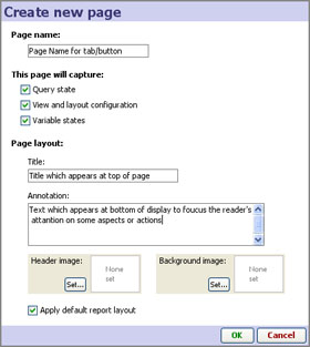 | Page name: this name appears on a report tab at the top of the display, or a button on the Sidebar Reports Panel if you provide access to Report pages there. Title: the title text that will appear at the top of the page...you can edit this at any time Apply default report layout: If you leave this box ticked, Omniscope will hide the View Toolbars and increase the margins around the views for a cleaner display. If you wish to preserve the existing settings, untick this box. |
Once configured and named, each pre-defined, persistent Report page appears anytime the user clicks on the top report tab, or the button next to the Report page name in the Sidebar Reports Panel, or uses the Reports Navigator menu, which appears faintly in the bottom left corner of the display in Reports Mode (see Using the Reports Navigator below).
The Main Toolbar Page menu commands provide many options useful for creating self-explanatory Report Pages. The commands on this menu can be used to configure many aspects of the current display, whether that display will eventually be converted to a persistent Report Page or not. If you make changes to the current view using Page menu commands, then close and save the file, it will next open with those changes preserved in the current display.
| Page > menu commands can be used to: You can also tick/untick the options to display or hide the Main Toolbar and the View Toolbars on open views of the page. Toolbars are usually hidden if Report Page users are not expected to access the options available on them. Even when hidden, the Main Toolbar comes back into view whenever the user hovers the mouse near the top of the display. |
Page > menu commands apply to each Report page individually, and any changes must be Committed to become a persistent change, or Reverted to return the Report page to its default configuration/layout. For options covering aspects of the look and feel of Report pages that apply to more then one page, see the introduction to the Appearance [436] command menu.
The Reports Navigator menu appears in the lower left-hand corner of the display whenever Omniscope is in Reports Mode, meaning displaying a persistent Report Page. The Reports Navigator is faint until you mouse over it, at which point it appears clearly, with forward and back arrows pointing to either side of a reports document icon. Clicking on the forward or back arrows cycles through all the Report Pages already configured in the file. The same list as can be seen in the Side Bar Reports (or some other name if you have renamed the Reports heading) panel and under the Main Toolbar Reports Navigation section.
Clicking on the Reports Navigator document icon at lower left reveals a menu listing a number of report navigation, creation, layout and reset options.
 | Start; Next; Previous; Go to page...used to cycle through the Reports Pages already configured in the file. Administer all pages sub-menu: Commit all modified pages- makes all changes which you have made to your Report Pages persistent Revert all modified pages- returns all Reports Pages to their last persistent configuration Delete all pages- deletes all Report Pages currently configured |
If the Commit and Revert modifications commands are solid, rather than greyed-out, it means that you have modified the current Report Page and must now either overwrite the previous settings with the new ones (Commit) or return the report to its original look, leaving the original settings unchanged (Revert). If the name of the Report Page is showing in red on the top report tab, this also means that you should either Commit or Revert your changes. If you have chosen to show the Side Bar Reports panel, these buttons also show in the Side Bar under the current Report Page whenever changes have been made to the current page, and the report titles will show in red until changes are either Committed or Reverted.
| Tools sub-menu: Tick or un-tick to Show or Hide various toolbars. Note that these changes apply to the current Report Page only, and only if the modifications are Committed to make them persistent. |
Reset Layout - returns the layout of the current Report Page to the default, with all the optional Show/Hide settings set to Show
Save file as... opens the Export file wizard [568]with the tab set to .IOK/.IOM files.
Exit Report: - exits from Reports Mode and the Report Navigator menu disappears. Remember that it is usually better to Exit Reports Mode if not modifying existing Reports Pages. You can also Exit Reports Mode from the Main Toolbar Reports menu (see below) or from the Side Bar Reports Panel if you are displaying reports there.
Commands required to manage all configured Report pages are available from the Main Toolbar Reports menu. In addition to many of the same commands as are available on the Reports Navigator menu, the Main Toolbar Reports menu includes commands such as Commit and Revert all modified pages that operate on all Report Pages simultaneously. When the Reports menu is opened, the title of the current Report Page is shown at the top in bold italics.
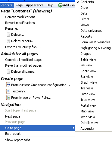
For more detail, see the sections documenting the Main Toolbar Report [566]s and Page [567] command menus
This refers to the functionality allowing Report pages to be organised into named sections (or "groups"). To date, Report page organisation has been implemented only in the Sidebar Reports panel. To show the Reports panel, the right-hand Sidebar must be showing. However, the Sidebar Reports panel is not displayed by default.
Use the Sidebar button on the Main Toolbar to change this. Then, ensure the Reports Panel is ticked for display using the Devices drop-down on the Sidebar toolbar. When the Sidebar Reports Panel is displayed, the Report page tabs across the top of the display will disappear unless they have been explicitly shown. You can explicitly hide/show the Report Page tabs using Main Toolbar: Tab > Tab settings > Tab bar option. For more information, see the Appearance menu [569]commands.
The Sidebar Reports Panel must be expanded to show the Create new button at the bottom of the panel. Expand/collapse each device by clicking its title. Click Create new, choose Section and enter the section name when prompted. Drag the sections and Report Page titles around to achieve the desired structure.
To manage existing section titles, click the black triangle on the right to show a drop-down menu, allowing you to rename or delete each section grouping.
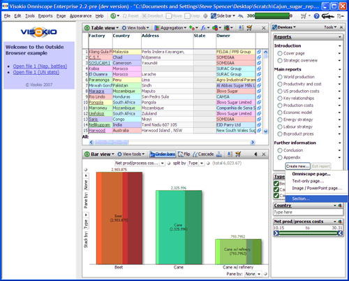
Applies to version 2.4 only
Omniscope enables you to deliver interactive, data-rich, visual presentations rather than dull, complex spreadsheets and/or static, non-interactive presentation slides. Omniscope also offers extensive options for branding your file, displaying advertising, focusing the end users' navigation options, and changing the layout, themes and colouring to match your organisation's standards for internal and external documents.
Commands/options relating to most of the elements of the display of pages/tabs in a given file are found under the Main Toolbar Appearance and Help menus. This page covers only two of the most commonly-used options; Branding and View restrictions. See Commands Reference 2-4 > Appearance [569]for a complete overview of commands on the Appearance sub-menu.
{Omniscope Professional & Enterprise only} The Branding sub-menu provides options to configure either of two informational pop-up screens presented on opening and closing a given file. It also provides the option to change the corner logo display from 'Visokio' to a logo of your own (with a link back to your own page), and to display banner advertising images and links in your downloadable Omniscope files.
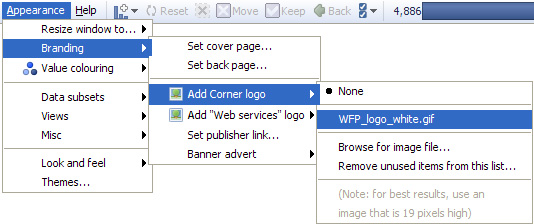
There are two pop-up informational screens you can configure:
The Add Corner logo, Add Web Services menu logo, and Set publisher link options enable data publishers to further brand their files. The Banner advert sub-menu enables publishers to add advertising images and links to their files to fully integrate with the commercial aspects of their business. For more information, see Appearance Menu [569] and Advertising Options. [570]
Note: The Help page and banner advertising displays are currently the same for the working display and all the Report Pages in the file, rather than configurable for each Report Page. This may change in future versions. To edit the file specific Help Page, see Help > Create/Edit help page.
Clicking on the option to configure a Cover and Back informational screens launches a Set Page dialog that accepts your inputs from you. The dialogs used to create the Cover and Back informational pages are both similar to the one shown below:
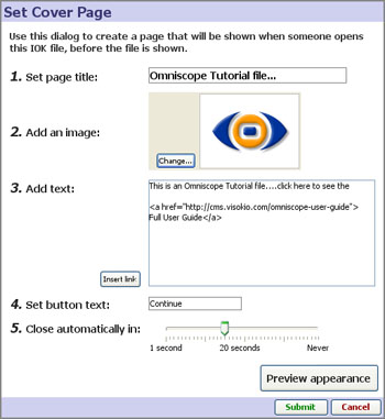
Note: Both information screens support some aspects of HTML text formatting, such as <b>, <i> etc. Currently, informational screens behave differently to the file-specific Help Page, which does not require hard returns and can be re-sized directly in preview mode.
For any given data set, one or more of Omniscope's 14 different views may not be needed to best depict the data set and support user interaction. It may be that the data does not contain any fields (columns) useful to plot against other fields in the Graph View. Some files could have so many different unique Category values in different fields that the Tree View becomes slow to open and use. Whether for these or other reasons relating to simplifying the file, it is possible to hide selected views from the users' View Chooser menus by unticking the view on the list displayed under Appearance > Views > {view restrictions}:
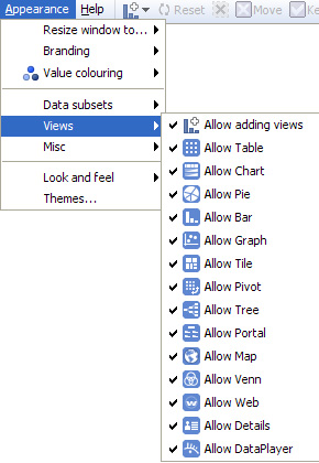
In addition to logos/background images and font selection, all the colours associated with an file can be managed using the options available under Appearance > Themes. There is a library of predefined Themes, and you also create your own combination of corporate colours and save the settings as your own named Theme which you can share with others. More on managing Themes [571].
Applies to Omniscope 2.4 only.
Themes are combinations of display settings you can change under Appearance > Look and Feel. These settings control most of the visible aspects of each file, outside of the controls available within individual views. By default, a built-in style called Default is used for every file. A menu of alternative pre-defined themes is available Appearance > Themes. You can see the different colouring effects by changing the style applied to the open file.
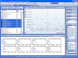 Ice Blue | 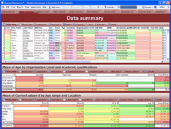 Bordeaux | 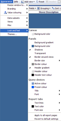 | |
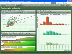 Forest | 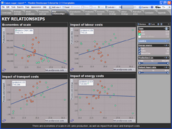 Darth Vader |
Create a corporate style corresponding to your corporate colours and general style of presentation, using a combination of official logos, font settings, colours and effects, which you can define using Appearance > Look and Feel. Once you are satisfied with all the settings, name and save your official style preset and it will become a new option on your Appearance > Themes menu. You can also copy this customised style preset to others in your organisation (see below), so that the official corporate preset is available in the same menu to everyone configuring files.
If you change any settings relative to the current style preset, the Preset selection drop down will show that the new altered preset is not saved. Click Save to give a name to the newly-modified style preset and save it to your installation, from which it will be available for future use, and transferable in the form of an .XML file you can copy across machines.
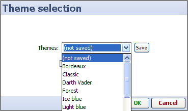 The settings corresponding to the new style preset are saved in a local .XML file named {YourPresetName}.XML. Anyone who creates a new file from an existing file can use the same style preset, which is part of the file. However, anyone creating a new file will not have access to the custom corporate style unless it is first copied to their machine.
Currently, to make a style preset you have defined available to others, you need to find the file called {YourPresetName}.XML on your machine, send a copy of this file to others needing to originate (not view) files with his preset, and tell them the location on their machine to copy this file so that it will be available to them whenever they create a new Omniscope file.
The location to find/copy the .XML style preset files varies by version of Omniscope and your version of Windows, as described below:
Vista:
C:\Users\UserName\AppData\Local\VirtualStore\Program Files\Visokio Omniscope\UserThemes
Windows XP:
C:\Program Files\Visokio Omniscope\UserThemes
If your system is set to hide system-related files and folders, you may not see the above locations until you change this setting:
1. Open the folder options in Windows:
Windows XP:
Open menu [START] > Settings > Control Panel > Folder options
Windows Vista:
Open menu [START] > Control Panel > Appearance and Personalisation > Folder options
2. Click on the View tab and enable the option 'Show hidden files and folders'.
DataPlayer is no longer being developed. To use, you must enable Settings > Advanced > Show legacy features.
The Omniscope DataPlayer View is a combined viewer and workspace that enables anyone to create exportable, interactive files we call DataPlayers. Using the DataPlayer View, some or all of the data in an Omniscope project file can be encapsulated in one or more Flash .SWF files combining the data, dynamic visualisations and query devices. DataPlayers can be embedded into offline documents (PowerPoint, Excel, Adobe Acrobat) and web pages with full interactivity. Flash is universally-accessible and does not require users to have the the Omniscope free Viewer installed to interact with and filter the data in real time.
Note: Due to limitations in Flash, DataPlayers can not yet be scaled up to include millions of rows as Omniscope files can. Although the upper limit is increasing over time, it currently can be difficult to get good performance in DataPlayers with over about 15,000 rows. DataPlayer scalability and performance will be increased dramatically in future releases. For more information, see KnowledgeBase article on DataPlayer scaling and performance [76].
The DataPlayer View is opened like any other, using the Add View menu on the Main Toolbar, or by switching from another view. Ticking the option Open in new window at the bottom of the Add View menu will allow you to manage the DataPlayer window independently. It is good practise to create a separate reporting tab for the DataPlayer View, which aids in creating DataPlayers and refreshing them later on. Note that under the Appearance menu, you can choose either Tabbed (one view type per tab in the single DataPlayer file, or Simultaneous, multiple ('dashboard') views for a given DataPlayer.
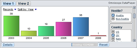
Upon opening a DataPlayer View, Omniscope will attempt to generate a Bar View DataPlayer using the Filtered data (IN) data set.
Warning: If you have more than 10-15,000 records in the filtered IN data set, current limitations in Flash may interfere with full rendering of the initial DataPlayer. It is best to first define either an Aggregation or a Named Query (or both) such that the number of records to be encapsulated in the DataPlayers is reduced to under about 15,000 depending on row count and data complexity.
The Side Bar filter devices and ordering settings showing when the DataPlayer View is opened are replicated in the DataPlayer filter panel which by default is on the right side of the DataPlayer. Once the initial Bar View DataPlayer is generated, you will notice the various interactive elements of the DataPlayer. Clicking on the filters in the side panel reduces the record count, as displayed in the barometer at the bottom. Clicking the Reset button restores all the records in the defined data set. Clicking on the details button displays (potentially aggregated) record level details (in an expandable table) which opens at record level to display all fields as configured.
Using the menu items available on the DataPlayer View Toolbar (see below), you can refine this opening DataPlayer, add other DataPlayer view types, and change the Omniscope Side Bar filter settings to influence the filter panel generated in the DataPlayer(s) you are creating.
Caution: The DataPlayers displayed in the DataPlayer View are fully interactive, and thus it is possible to set filters, change selection drop-downs etc. just as end-users of the DataPlayer will. However, these changes are NOT PERSISTENT. The next time the DataPlayer View is opened and the DataPlayer re-generated, all settings will revert to the settings established in the View Toolbar settings menus, described briefly below and in detail in the in the DataPlayer View [427] reference section.
Refreshing the data in the Omniscope file, then updating the DataPlayer View will create an updated Flash 'dashboard' file containing the latest data, which can be posted to the web or exported into existing documents, over-writing the previous versions.
Like other View Toolbars, the DataPlayer View Toolbar displays many of the standard menus, such as the window View picker, Data Subset, Aggregate and View tools menus, but also various specialised drop-down menus containing options for adding and configuring DataPlayers. Given the scaling limitations of DataPlayers, it is sometimes necessary to define Named Queries and/or aggregations in the DataPlayer view to reduce the record count sufficiently to allow one or more DataPlayers to be generated.
![]()
In addition to the standard View Toolbar menu items, the specialised menus on the DataPlayer View Toolbar include:
This section is just a brief introduction to the process of creating and exporting interactive DataPlayers from defined data-subsets and filter settings in your Omniscope files. More detail on all the myriad configuration options for all view types is available in the Views Reference DataPlayer View section [427].
Below is an index to all the drop-down command menus accessed from the Main Toolbar [441] for version 2.5. For information on commands and options related to specific Views and View Toolbars, please consult the Guide to Views. [21] If you're still using version 2.4, please see the command reference for 2.4 [481]. If you're accustomed to Omniscope 2.4, and can't find a command in version 2.5, see this guide to changes [572].
Main Toolbar Commands - version 2.5
Click for an overview of the Main Toolbar in version 2.5 [441] Click on the links below for more detail on the section containing the command(s) you are seeking. |File [442]|Data [443] |Tab [444] |Layout [25] |Toolbars [445] |Settings [446] |Help [447]| | |
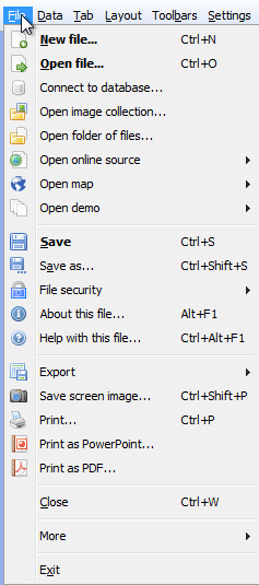 | File menu [442]
|
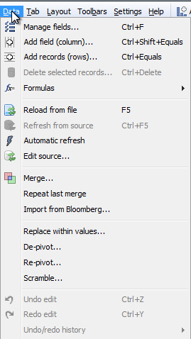 | Data menu [443]Manage fields |
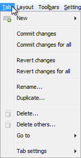 | Tab menu [444]New [444] |
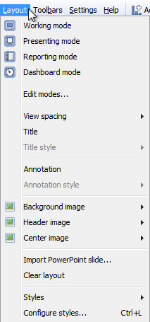 | Layout menu [25]Mode selection: [25] Working mode-------------------------- |
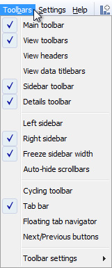 | Toolbars menu [445]Toolbar visibility: |
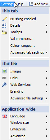 | Settings menu [446]This tab: [446] |
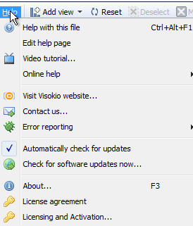 | Help menu [447]Help with this file - |
The Omniscope Main Toolbar contains both a series of drop-down command menus on the left and a selection of navigational command icons and functions to the right of the command menus used to explore and refresh Omniscope files. The command menu options on the Main Toolbar are generally not needed to navigate Omniscope files prepared by others. The number of icons and detail displayed will depend on the horizontal space available to Omniscope. Various Layout modes may hide the Main Toolbar unless the user hovers their mouse near the top of the display.
![]()
| Add View - opens a new View window | |||
| Reset - returns all records to the filtered IN subset | Working Mode - layout for configuring files | ||
| Deselect - removes all selections | Presentation Mode - layout for presentations | ||
| Move - selected records to the filtered OUT subset | Reporting Mode - layout for printing | ||
| Keep - selected records in the filtered IN subset | Dashboard Mode - layout for refreshable displays | ||
| Back - to the previous display | Zoom - adjusts display resolution/font size | ||
| Colour by - choose global colouring option | Help page - launches file-specific help screen | ||
| Details - display field values for selected record set | File close - closes the open file | ||
OUT (174), and Selected (1) record (row) counts | Expand/Show Labels - expands and wraps Main Toolbar to display labels | ||
See the section below for more detail on Main Toolbar commands
The left side of the Main Toolbar contains all the top-level command menus. When no Omniscope data file is loaded, the Main Toolbar displays only these command menus and the Welcome Screen [389]. File menu [442]: importing/refreshing, saving, exporting and printing data, maps and image sets. Data menu [443]: managing data columns (fields) and values within categories, adding new columns & rows and changing data orientation (de-pivot and re-pivot). Tab menu: [444] enable auto-refresh, change languages, set details display options, define links, image sets and web services related to the file. Layout menu: [25] create, modify and navigate Report pages. Toolbars menu: [574] modify aspects of the workspace or current Report page. Settings menu: [446] add branding and modify/simplify most aspects of the colouring, look and feel of the file. Help menu: [447] create file-specific help screen, access learning resources, send bug reports/suggestions, check for updates and licensing status (if these services are not working, consult the KnowledgeBase section on Proxy Settings [575]).
Complete documentation of all the commands on these menus can be accessed from the Commands Reference [440] page or by following the links above. | Add View menu: |
| |||||||||||||||||||||||
Reset - Omniscope files contain flat tables of structured data organised into records (rows) and fields (columns). Navigating an Omniscope file usually involves either setting Side Bar filters, or Selecting plus either Move or Keep operations to focus on only a certain data subset. The Reset button removes all of the filtering criteria you may have expressed, and returns the current display views to show all the records in the Filtered IN universe. It is very important to always Reset your data before filtering, so that all qualifying records will be considered in your subsequent query. Unless you configure them otherwise, tabs remember their queries/data subsets, so if you want a Report Page to open showing all the data, make sure to Reset all the filters and commit the changes before you save the file. Note: On the Side Bar filter devices it is possible to reset each filter individually, and if a Side Bar filter device is set to Freeze, that filter's settings will survive a global Reset. | ||
Deselect - Removes all records from the Selected data subset and greys-out the option to do Move or Keep operations on selected records. Omniscope power query filtering directly on views (as opposed to Side Bar filtering) involves 4 basic mouse operations: Select (or Deselect), followed by Move or Keep, and then perhaps a Reset. Every view provides ways of selecting one or more records using just the mouse. In most views, you can also Deselect by clicking again on one or more of the selected areas or groups of records. It is not necessary to use this global Deselect on the Main Toolbar unless you wish to clear all selections made simultaneously. | ||
| Move - Selecting records is a precursor to deciding whether to Move the selected records, i.e. filtered OUT of further consideration. If you are working from a view of the filtered IN data subset, the grey Move command moves all selected records OUT of consideration, where they stay until they are returned or the display is Reset. The barometer will give you a preview of this on the left side, where selected IN records to be moved will be highlighted. If you are working from the filtered OUT data subset, the display will change the colour of the Move icon to blue, since moving records from the filtered OUT subset will return them to the filtered IN subset. The barometer will show you the selected OUT records highlighted on the right side. If you are working from a view set to display ALL Data, the barometer will show you the effect of Moves and Keeps, but that specific view will not update as a result, since views showing ALL Data always display all records regardless of whether they are filtered IN or OUT. | ||
| Keep- the opposite of Move, the Keep command keeps only the selected records in the filtered IN subset, and moves all other unselected records to the filtered OUT subset. If you are working from a view displaying the filtered OUT subset, the Keep icon will change colour to grey, since the effect will be toKeep the selected records in the filtered OUT subset. If you are working from a view set to display ALL Data, the barometer will show you the effect of Moves and Keeps, but that specific view will not update as a result, since views showing ALL Data always display all records regardless of whether they are filtered IN or OUT. | ||
| Back- similar to a browser, if you have performed a filtering operation, you can go back to the previous query state(s) at any time by pressing the Back button. | ||
| ||
| Queries - this drop-down menu is used to manage defined data subsets associated with Named Queries. Using this menu you can name empty queries ( e.g "Basket" or "Errors") to collect records you add, or you can define complex queries as re-usable Named Queries using patterns of Side Bar filter settings. Each Named Query defined is added to the data subsets that can be displayed in most views. Detailed documentation of the use of the commands on this menu is here [22]. | ||
| Barometer - this very useful indicator depicts the top level query state (records IN and OUT, with currently selected subsets counts) at any given time. In this example, the data set contains 4,886 total records (rows), of which 4,292 remain in the filtered IN subset, and 594 have been moved to the filtered OUT subset. In addition, 1,719 records have been selected, and the currently highlighted single record is among those selected. Always keep an eye on the barometer before initiating new filtering/queries to ensure that you have Reset (or gone Back) to the correct IN subset. | ||
| Auto-refresh settings - Omniscope files can have other Omniscope files as data sources. Activated Omniscopes can refresh the data in an open .IOK/.IOM file from the data in another .IOK/.IOM file accessible over a network. The Auto-refresh drop down menu is revealed by activating the Automatic refresh option from the Tools menu [576]. Once revealed, this menu allows all aspects of the refresh process to be configured, as described here. [415] There is an option to display a Pause/Resume button (see below). | ||
| Pause/Resume (auto-refresh)- Auto-refresh settings options include displaying a Pause/Resume auto-refresh button on the Main Toolbar. | ||
| | File-specific help screen - click to what the owner of a given file may have written to help users understand more about the file. If you are configuring a file for others, the content of this screen is composed from Help > Edit Help screen. | |
| Corner logo - if you are publishing or re-publishing .IOK/.IOM files, you can replace this logo and link with your own. See Appearance > Branding > Add Corner Logo and Set Publisher link (for best results, use a logo 19 pixels high). | ||
| Close file - click here to close the .IOK/.IOM file currently open. Once the data file is closed, the screen will display the Omniscope opening desktop, which includes links to previously opened files, as well as learning resources, embedded demos and other useful resources. | ||
Relates only to version 2.4
The Omniscope Main Toolbar contains both a series of drop-down command menus on the left and a selection of navigational command icons and functions used to explore and refresh Omniscope files to the right of the command menus. The command menu options are generally not needed to navigate Omniscope files prepared by others.
![]()
Immediately to the right of the Help command is the Add View drop down menu, used to add an additional view to the current display. To remove a view from the display, click on the [X] in the upper right hand corner of the view. To change a window from one view to another, click on the view name and select the view you want from the drop-down menu. If you want to add a view showing another data subset, you can select it using the Data Subset drop-down to the right of the view name in each View Toolbar.There is no upper limit on the number of views you can open in Omniscope, but display screen size limitations encourage using multiple tabbed Report Pages to display different combinations of views, rather than crowding the working display with too many open views. More on creating Report Pages [435].
| File [577]| Edit [578] | Tools [579] | Reports [566] | Page [567] | Appearance [569]| Help [580] | The left side of the Main Toolbar contains all the top-level command menus. When no .IOK/.IOM data file is loaded, the Main Toolbar displays only the command menus. File menu [577]: importing/refreshing, saving, exporting and printing data, maps and image sets. Edit menu: [578] managing data columns (fields) and values within categories, adding new columns & rows and changing data orientation (de-pivot and re-pivot). Tools menu: [579] enable auto-refresh, change languages, set details display options, define links, image sets and web services related to the file. Reports menu: [566] create, modify and navigate Report pages. Page menu: [567] modify aspects of the workspace or current Report page. Appearance menu: [569] add branding and modify/simplify most aspects of the colouring, look and feel of the file. Help menu: [580] create file-specific help screen, access learning resources, send bug reports/suggestions, check for updates and licensing status.
Complete documentation of all the commands on these menus can be accessed from the Commands Reference 2.4 [481] page or by following the links above. | Add View menu: |
|
Whenever a data file is loaded, to the right of the command menus, the Main Toolbar also displays a selection of navigational command icons and functions used to explore and refresh Omniscope files:
![]() Reset - Omniscope files contain flat tables of structured data organised into records (rows) and fields (columns). Navigating an Omniscope file usually involves either setting Side Bar filters, or Selecting plus either Move or Keep operations to focus on only a certain data subset. The Reset button removes all of the filtering criteria you may have expressed, and returns the current display views to show all the records in the Filtered IN universe. It is very important to always Resetyour data before filtering, so that all qualifying records will be considered in your subsequent query. Unless you configure them otherwise, Report Pages remember their queries/data subsets, so if you want a Report Page to open showing all the data, make sure to Reset all the filters and commit the changes before you save the file. Note: On the Side Bar filter devices it is possible to reset each filter individually, and if a Side Bar filter device is set to Freeze, that filter's settings will survive a globalReset.
Reset - Omniscope files contain flat tables of structured data organised into records (rows) and fields (columns). Navigating an Omniscope file usually involves either setting Side Bar filters, or Selecting plus either Move or Keep operations to focus on only a certain data subset. The Reset button removes all of the filtering criteria you may have expressed, and returns the current display views to show all the records in the Filtered IN universe. It is very important to always Resetyour data before filtering, so that all qualifying records will be considered in your subsequent query. Unless you configure them otherwise, Report Pages remember their queries/data subsets, so if you want a Report Page to open showing all the data, make sure to Reset all the filters and commit the changes before you save the file. Note: On the Side Bar filter devices it is possible to reset each filter individually, and if a Side Bar filter device is set to Freeze, that filter's settings will survive a globalReset.
![]() Deselect - Removes all records from the Selected data subset and greys-out the option to do Move or Keep operations on selected records. Omniscope power query filtering directly on views (as opposed to Side Bar filtering) involves 4 basic mouse operations: Select (or Deselect), followed by Move or Keep, and then perhaps a Reset. Every view provides ways of selecting one or more records using just the mouse. In most views, you can also Deselect by clicking again on one or more of the selected areas or groups of records. It is not necessary to use this global Deselect on the Main Toolbar unless you wish to clear all selections made simultaneously.
Deselect - Removes all records from the Selected data subset and greys-out the option to do Move or Keep operations on selected records. Omniscope power query filtering directly on views (as opposed to Side Bar filtering) involves 4 basic mouse operations: Select (or Deselect), followed by Move or Keep, and then perhaps a Reset. Every view provides ways of selecting one or more records using just the mouse. In most views, you can also Deselect by clicking again on one or more of the selected areas or groups of records. It is not necessary to use this global Deselect on the Main Toolbar unless you wish to clear all selections made simultaneously.
![]() Move - Selecting records is a precursor to deciding whether to Move the selected records, i.e. filtered OUT of further consideration. If you are working from a view of the filtered IN data subset, the grey Move command moves all selected records OUT of consideration, where they stay until they are returned or the display is Reset. The barometer will give you a preview of this on the left side, where selected IN records to be moved will be highlighted. If you are working from the filtered OUT data subset, the display will change the colour of the Move icon to blue, since moving records from the filtered OUT subset will return them to the filteredIN subset. The barometer will show you the selected OUT records highlighted on the right side. If you are working from a view set to display ALL Data, the barometer will show you the effect of Moves and Keeps, but that specific view will not update as a result, since views showing ALL Data always display all records regardless of whether they are filtered IN or OUT.
Move - Selecting records is a precursor to deciding whether to Move the selected records, i.e. filtered OUT of further consideration. If you are working from a view of the filtered IN data subset, the grey Move command moves all selected records OUT of consideration, where they stay until they are returned or the display is Reset. The barometer will give you a preview of this on the left side, where selected IN records to be moved will be highlighted. If you are working from the filtered OUT data subset, the display will change the colour of the Move icon to blue, since moving records from the filtered OUT subset will return them to the filteredIN subset. The barometer will show you the selected OUT records highlighted on the right side. If you are working from a view set to display ALL Data, the barometer will show you the effect of Moves and Keeps, but that specific view will not update as a result, since views showing ALL Data always display all records regardless of whether they are filtered IN or OUT.
![]() Keep - the opposite of Move, the Keep command keeps only the selected records in the filtered IN subset, and moves all other unselected records to the filtered OUT subset. If you are working from a view displaying the filtered OUT subset, the Keep icon will change colour to grey, since the effect will be toKeep the selected records in the filtered OUT subset. If you are working from a view set to display ALL Data, the barometer will show you the effect of Moves andKeeps, but that specific view will not update as a result, since views showing ALL Data always display all records regardless of whether they are filtered IN or OUT.
Keep - the opposite of Move, the Keep command keeps only the selected records in the filtered IN subset, and moves all other unselected records to the filtered OUT subset. If you are working from a view displaying the filtered OUT subset, the Keep icon will change colour to grey, since the effect will be toKeep the selected records in the filtered OUT subset. If you are working from a view set to display ALL Data, the barometer will show you the effect of Moves andKeeps, but that specific view will not update as a result, since views showing ALL Data always display all records regardless of whether they are filtered IN or OUT.
![]() Back - similar to a browser, if you have performed a filtering operation, you can go back to the previous query state(s) at any time by pressing the Back button.
Back - similar to a browser, if you have performed a filtering operation, you can go back to the previous query state(s) at any time by pressing the Back button.
![]() Controls - this drop-down menu controls display of the two Sidebars, as well as the Cycling Toolbar. For more detail, see the Controls [484] subsection.
Controls - this drop-down menu controls display of the two Sidebars, as well as the Cycling Toolbar. For more detail, see the Controls [484] subsection.
![]() Barometer - this very useful indicator depicts the top level query state (records IN and OUT, with currently selected subsets counts) at any given time. In this example, the data set contains 4,886 total records (rows), of which 4,292 remain in the filtered IN subset, and 594 have been moved to the filtered OUT subset. In addition, 1,719 records have been selected, and the currently highlighted single record is among those selected. Always keep an eye on the barometer before initiating new filtering/queries to ensure that you have Reset (or gone Back) to the correct IN subset.
Barometer - this very useful indicator depicts the top level query state (records IN and OUT, with currently selected subsets counts) at any given time. In this example, the data set contains 4,886 total records (rows), of which 4,292 remain in the filtered IN subset, and 594 have been moved to the filtered OUT subset. In addition, 1,719 records have been selected, and the currently highlighted single record is among those selected. Always keep an eye on the barometer before initiating new filtering/queries to ensure that you have Reset (or gone Back) to the correct IN subset.
![]() Queries - this drop-down menu is used to manage defined data subsets associated with Named Queries. Using this menu you can name empty queries ( e.g "Basket" or "Errors") to collect records you add, or you can define complex queries as re-usable Named Queries using patterns of Side Bar filter settings. Each Named Query defined is added to the data subsets that can be displayed in most views. Detailled documentation of the use of the commands on this menu is here [22].
Queries - this drop-down menu is used to manage defined data subsets associated with Named Queries. Using this menu you can name empty queries ( e.g "Basket" or "Errors") to collect records you add, or you can define complex queries as re-usable Named Queries using patterns of Side Bar filter settings. Each Named Query defined is added to the data subsets that can be displayed in most views. Detailled documentation of the use of the commands on this menu is here [22].
![]() Auto-refresh settings - Omniscope files can have other Omniscope files as data sources. Activated Omniscopes can refresh the data in an open .IOK/.IOM file from the data in another .IOK/.IOM file accessible over a network. The Auto-refresh drop down menu is revealed by activating the Automatic refresh option from the Tools menu [576]. Once revealed, this menu allows all aspects of the refresh process to be configured, as described here. [415] There is also an option to display a Pause/Resume button (see below).
Auto-refresh settings - Omniscope files can have other Omniscope files as data sources. Activated Omniscopes can refresh the data in an open .IOK/.IOM file from the data in another .IOK/.IOM file accessible over a network. The Auto-refresh drop down menu is revealed by activating the Automatic refresh option from the Tools menu [576]. Once revealed, this menu allows all aspects of the refresh process to be configured, as described here. [415] There is also an option to display a Pause/Resume button (see below).
![]() Pause/Resume (auto-refresh) - Auto-refresh settings options include displaying a Pause/Resume auto-refresh button on the Main Toolbar.
Pause/Resume (auto-refresh) - Auto-refresh settings options include displaying a Pause/Resume auto-refresh button on the Main Toolbar.
![]() File-specific help screen - click on this help icon to see what the publisher or re-publisher of a given file may have written to help users understand more about the file. If you are configuring a file for others, the content of this screen may be composed from Help > Edit Help screen.
File-specific help screen - click on this help icon to see what the publisher or re-publisher of a given file may have written to help users understand more about the file. If you are configuring a file for others, the content of this screen may be composed from Help > Edit Help screen.
![]() Corner logo - if you are publishing or re-publishing .IOK/.IOM files, you can replace this logo and link with your own. See Appearance > Branding > Add Corner Logo and Set Publisher link (for best results, use a logo 19 pixels high).
Corner logo - if you are publishing or re-publishing .IOK/.IOM files, you can replace this logo and link with your own. See Appearance > Branding > Add Corner Logo and Set Publisher link (for best results, use a logo 19 pixels high).
![]() Close file - click here to close the Omniscope file currently open. Once the data file is closed, the screen will display the Omniscope opening desktop, which includes links to previously opened files, as well as learning resources, embedded demos and other useful resources.
Close file - click here to close the Omniscope file currently open. Once the data file is closed, the screen will display the Omniscope opening desktop, which includes links to previously opened files, as well as learning resources, embedded demos and other useful resources.
Relates only to version 2.4 and prior
The Controls drop-down menu is located on the Main Toolbar to the left of the Barometer.
Show right/left Sidebar - displays one or both Side Bars. By default, all filter Devices are initially displayed on the right side bar. To move filter Devices to the left Side Bar, open the left Side Bar and use the Devices drop down on the left Side Bar to tick which devices you want to move from the right to left Side Bar. Using Side Bars [483] Auto-hide main toolbar - ticking this option will cause the Main Toolbar to retract for all Report Tabs and the workspace, unless the mouse is hovered above the Report tabs at the top of the screen. This is often useful when simplifying the page layout for live presentations. This option can also be set on an individual Report Page basis by unticking the Show main toolbar option at the bottom of the Page menu [581], then committing the change on each Report Page tab for which you do not want the Main Toolbar displayed. |
Cycling toolbar - the Cycling Toolbar contains the setting for automatically cycling through Records, Values and Reports, introducing a degree of automation in the display of the data and images in the file. When set to Hide, the Cycling Toolbar will not display. The Auto-show option will enable display of the Cycling toolbar when the mouse hovers at the bottom of the screen. The Show option will display the Cycling Toolbar at all times. Using the Cycling Toolbar [556]
Relates only to version 2.3 and earlier.
The left side of the Main Toolbar contains all the top-level command menus. When no Omniscope data file is loaded, the Main Toolbar displays only the command menus. These commands are generally not needed to navigate an Omniscope file prepared for you by someone else. Documentation of all the commands on these menus can be accessed from the Commands Reference [481] page or by following the links below:
| File [582]| Edit [26] | Tools [583] | Reports [584] | Page [34] | Appearance [585]| Help [586] |
Whenever an Omniscope data file is loaded, to the right of the command menus, the Main Toolbar also displays a selection of navigational command icons and functions used to explore Omniscope files:
![]()
![]() Add View -Used to add an additional view to the current display. To remove a view from the display, click on the [X] in the upper right hand corner of the view. To change a window from one view to another, click on the view name and select the view you want from the drop-down menu. If you want to add a view showing another Universe, click on the Show other data universes option to display a grid of all views and universes. There is no upper limit on the number of views you can open in Omniscope, but display screen size limitations encourage using multiple Report Pages to display different combinations of views, rather than crowding the working display with too many open views. More on creating Report Pages [435].
Add View -Used to add an additional view to the current display. To remove a view from the display, click on the [X] in the upper right hand corner of the view. To change a window from one view to another, click on the view name and select the view you want from the drop-down menu. If you want to add a view showing another Universe, click on the Show other data universes option to display a grid of all views and universes. There is no upper limit on the number of views you can open in Omniscope, but display screen size limitations encourage using multiple Report Pages to display different combinations of views, rather than crowding the working display with too many open views. More on creating Report Pages [435].

![]() Reset - Omniscope files are flat tables of data, with records (rows) and fields (columns). One of the objectives of navigating an Omniscope file is to select and focus on only a certain subset of records (rows), rather than all the records in the file. The Reset button removes all of the filtering criteria you may have expressed, and returns the current display views to show all the records in the IN universe. It is very important to always reset your data before filtering, so that all qualifying records will be considered in your subsequent query. Unless you say otherwise, Report Pages remember their queries, so if you want a Report Page to open showing all the data, make sure to Reset the views and commit the changes before you save the file.
Reset - Omniscope files are flat tables of data, with records (rows) and fields (columns). One of the objectives of navigating an Omniscope file is to select and focus on only a certain subset of records (rows), rather than all the records in the file. The Reset button removes all of the filtering criteria you may have expressed, and returns the current display views to show all the records in the IN universe. It is very important to always reset your data before filtering, so that all qualifying records will be considered in your subsequent query. Unless you say otherwise, Report Pages remember their queries, so if you want a Report Page to open showing all the data, make sure to Reset the views and commit the changes before you save the file.
![]() Deselect - Removes all records from the blue SELECTION universe, and greys-out the option to do Move or Keep operations on selected records. Omniscope filtering using power queries depends on 4 basic operations: Select (or Deselect), followed by Move or Keep, and perhaps a Reset. Every view provides ways of selecting one or more records using just a mouse. In most views, you can also Deselect by clicking again on one or more of the selected areas or groups of records. It is not necessary to use the global Deselect on the Main Toolbar unless you wish to clear all selections.
Deselect - Removes all records from the blue SELECTION universe, and greys-out the option to do Move or Keep operations on selected records. Omniscope filtering using power queries depends on 4 basic operations: Select (or Deselect), followed by Move or Keep, and perhaps a Reset. Every view provides ways of selecting one or more records using just a mouse. In most views, you can also Deselect by clicking again on one or more of the selected areas or groups of records. It is not necessary to use the global Deselect on the Main Toolbar unless you wish to clear all selections.
![]() Move - Selecting/deselecting records is a precursor to deciding whether to Move the selected records OUT of further consideration. If you are working in the IN universe, the Move command moves all selected records OUT of consideration, where they stay until the display is Reset. If you are working from the OUT Universe, the display will change the colour of the Move icon to green, since moving records from the OUT Universe will return them to the green IN Universe. If you are working from the black ALL universe, the display will change the Move button, substituting OUT for Move, signifying that moving records from the ALL Universe places them in the OUT Universe, if they are not already there. Remember that the black ALL Universe always contains all records and does not change.
Move - Selecting/deselecting records is a precursor to deciding whether to Move the selected records OUT of further consideration. If you are working in the IN universe, the Move command moves all selected records OUT of consideration, where they stay until the display is Reset. If you are working from the OUT Universe, the display will change the colour of the Move icon to green, since moving records from the OUT Universe will return them to the green IN Universe. If you are working from the black ALL universe, the display will change the Move button, substituting OUT for Move, signifying that moving records from the ALL Universe places them in the OUT Universe, if they are not already there. Remember that the black ALL Universe always contains all records and does not change.
![]() Keep - the opposite of Move, if you are working in the IN Universe, the Keep command keeps only the selected records IN consideration, and moves all other unselected records OUT of consideration. If you are working from the OUT Universe, the display will change the colour of the Keep icon to red, since it will keep selected records in the OUT Universe and will return all others to the green IN Universe. If you are working from the black ALL Universe, the display will change the Keep button, substituting IN for Keep, signifying that keeping records from the ALL Universe places them in the IN Universe, if they are not already there. Remember that the Black ALL Universe always contains all records and does not change.
Keep - the opposite of Move, if you are working in the IN Universe, the Keep command keeps only the selected records IN consideration, and moves all other unselected records OUT of consideration. If you are working from the OUT Universe, the display will change the colour of the Keep icon to red, since it will keep selected records in the OUT Universe and will return all others to the green IN Universe. If you are working from the black ALL Universe, the display will change the Keep button, substituting IN for Keep, signifying that keeping records from the ALL Universe places them in the IN Universe, if they are not already there. Remember that the Black ALL Universe always contains all records and does not change.
![]() Back - like with a browser, you can go back to the previous display at any time by pressing Back.
Back - like with a browser, you can go back to the previous display at any time by pressing Back.
![]() Show Side Bar - clicking this icon gives you the option to show or hide the Side Bars on one or both sides of the current display. You can choose to display a Side Bar on the right, the left or both sides of the display. If you display both Side Bars, adding a device to one Side bar display will remove it from the other.
Show Side Bar - clicking this icon gives you the option to show or hide the Side Bars on one or both sides of the current display. You can choose to display a Side Bar on the right, the left or both sides of the display. If you display both Side Bars, adding a device to one Side bar display will remove it from the other.
![]() DataPlayer link - used to export data sets to Omniscope's companion application FeatureFinder (integrated as DataPlayer View in 2.4+). The separate application converts your data into interactive Flash .SWF DataPlayers suitable for embedding in web pages and offline documents such as PowerPoint, Adobe Acrobat .PDFs, Excel etc. DataPlayers in version 2.3 do not scale to more than about 5-10,000 typical records [76], so you may have to use Omniscope to divide your data set into smaller sets before exporting the data to convert as DataPlayers.
DataPlayer link - used to export data sets to Omniscope's companion application FeatureFinder (integrated as DataPlayer View in 2.4+). The separate application converts your data into interactive Flash .SWF DataPlayers suitable for embedding in web pages and offline documents such as PowerPoint, Adobe Acrobat .PDFs, Excel etc. DataPlayers in version 2.3 do not scale to more than about 5-10,000 typical records [76], so you may have to use Omniscope to divide your data set into smaller sets before exporting the data to convert as DataPlayers.
![]() Barometer - upon opening a file, it is useful to know how many records are in the data set. As you filter, it is useful to see how many records have been kept IN consideration, and how many moved OUT. The barometer is a visual gauge that shows the total, as well as the split between IN and OUT Universes. More on Data Universes [587]
Barometer - upon opening a file, it is useful to know how many records are in the data set. As you filter, it is useful to see how many records have been kept IN consideration, and how many moved OUT. The barometer is a visual gauge that shows the total, as well as the split between IN and OUT Universes. More on Data Universes [587]
![]() Basket - the basket is a 'parking place' where you can put selected records, such that they will stay there even if you Reset the display. At any time, you can open the Basket and see the records you have placed there.
Basket - the basket is a 'parking place' where you can put selected records, such that they will stay there even if you Reset the display. At any time, you can open the Basket and see the records you have placed there.
![]() Help screen - click on the help icon to see what the publisher or re-publisher of the file may have to say that will help you understand more about the file.
Help screen - click on the help icon to see what the publisher or re-publisher of the file may have to say that will help you understand more about the file.![]() Publisher logo/ link - if you are publishing or re-publishing an .IOK file, you can put your own logo here, and link it to your website. See Appearance > Branding > Add Corner Logo and Set Publisher link (for best results, use a logo 19 pixels high).
Publisher logo/ link - if you are publishing or re-publishing an .IOK file, you can put your own logo here, and link it to your website. See Appearance > Branding > Add Corner Logo and Set Publisher link (for best results, use a logo 19 pixels high).
The File > ... menu groups commands related to importing data from a file, reporting views/table(s) of a relational database, online 'cloud' data sources, folder of images, a folder of files (documents, music, videos), maps from our online library or a preconfigured demo file. The second section provides options for saving Omniscope files with a wide range of options. The third section provides options for exporting new files in Omniscope and other formats, exporting screen images form Omniscope, and printing Omniscope files in varous document formats.
| New file [397] - opens a dialog where you can specify how many rows and columns you need to start with. Generally, you should start small, except if you are planning to cut-and-paste data into the new Omniscope file, in which case you must specify enough rows and columns to receive the paste. Open file [400]- launches the Open file dialog, which looks like a Windows file browse window, but has some additional features and options on the right side. Navigate your directory structure and find the file you wish to load, e.g. an existing Omniscope IOK file, or a supported delimited data file; Excel XLS, CSV (comma separated value) or other common data file formats such as TSV, TXT etc. Connect to database [402] - launches the Database Connection Wizard that helps you connect to any ODBC/JDBC [588] compliant relational database and import/refresh the output of any SQL statement that returns a tabular data set. Open image collection [412] - imports a collection of image files and associated editable tags from a defined folder/location Open folder of files [411]- imports filenames, attributes, paths and associated editable tags from selected folders containing documents, and/or media files like music or video, with options to display the selected docments (PDF) or to edit tags and file names on media file libraries and export a playlist. Open online source [403] - Open map [401] - Open demo [390] - |
Applies to version 2.4 only
The File > Export > Export file(s) sub-menu provides many options for exporting some or all of the data, images and queries from the open Omniscope file for use by other applications, such as spreadsheets, or in the case of References and XML query files, by other Omniscope users with access to copies of the same IOK file.

Selecting File > Export > Export file(s) launches the Export Data wizard. Choosing File > Export > Export file(s) > Export References, > Export the images, and > Export XML query file also open the Export file wizard to the relevant tab.
The Export files wizard is a tabbed dialog that enables you to export data as a new Omniscope IOK file, an Excel XLS file, a list of references (values from one selected field/column) as a TXT file, a folder of images you have associated with (but not necessarily embedded into) the IOK file, or an Omniscope query as an XML file that can be opening by other Omniscopes to re-create the same view with the same data file. You change the type of file you want to export by selecting the appropriate tab at the top of the Export files wizard.
Selecting the Export Data tab will specify an Excel Workbook XLS file by default, but you can change the format of the exported data file to another supported format such as comma-separated value (CSV), tab-separated value (TSV) or an XML text data file (in Visokio schema [472]).
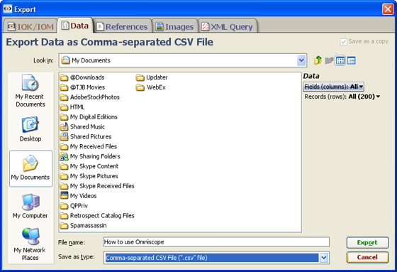
At the right side of the Export Data wizard, there are powerful options for specifying the fields (columns) and records (rows) to be exported. Untick any fields you do not want exported to the new file, and specify which data universe currently contains the records that you wish to export.
At any time, you can use the File > Save as or the Export Data wizard to create a new Omniscope IOK file from an existing one by selecting the first IOK tab on the Export Data wizard. In addition to specifying the fields and records you want to export, you also have several options to manage access and the refresh cycle for the new IOK file.
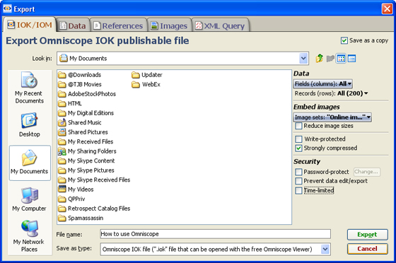
IOK files are already many times smaller than the equivalent spreadsheet file size. Strong compression reduces the size of IOK files even further, at the expense of requiring more memory and taking longer to save the file. Strong compression reduces CSV files much more than Zip compression, for example. You might use this if you are publishing or sending files via email or the web.
When creating new Omniscope IOK files, you can choose to save the new file using several options for managing access to the file, to the data inside the file, and the period of time for which the file will be valid. More on file security options. [439]
Sometimes you will want to export only a list of record (row) identifiers to share with others using Omniscope or other applications. Choosing the References tab in the Data Export dialog allows you to specify which field (column) you wish to export, and which Universe contains the records you wish to export.
{Version 2.3 and prior} For example, if you have saved a number of interesting records in the Basket, you would specify BASKET, rather than IN, SELECTION or ALL universes as the source of the records references to be exported.

Reference files are exported as single column TXT files, useful for importing/matching in to other applications or other Omniscopes to re-create the same list, perhaps with updated data, for co-workers or customers.
If you have associated an image set with a particular Omniscope file, the Export Data dialog will display an Images tab option. Selecting this tab allows you to create a new copy of the image folder, perhaps changing the size of the images to reduce the size of the files in which they will be embedded. If you have downloaded all online images associated with a file (by opening a Tile View showing the images, or using record cycling in the Details view, for example) you can export a copy of those images to a folder for local use.
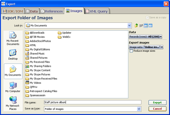
Note that the image set to be exported only needs to be associated with (but not necessarily embedded into) the current Omniscope file in order to use the Export Folder of Images option. If you are exporting an embedded image set that you have already reduced from the original sizes, Omniscope may warn you that it does not have access to the folder with the images at original size, and that the images in the new, exported folder will be of reduced size.
Any pattern of filter settings and history of Moves and Keeps can be saved as a named query, using an XML file only Omniscope can read and load as a query. The query may be the current active query, or any query associated with a Report Page defined in the file.
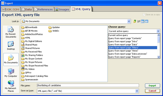
Exported queries can only be opened by other Omniscopes with open files that have the same fields present. There may be new records or changed data values in the version of the file importing the query, however. The export/import XML queries feature is used to permit others to quickly reproduce a data quality or screening views using the IN and OUT universes, perhaps on a daily basis as the data in each successive version of the Omniscope file changes.
The Data > menu groups commands for managing the underlying tabular data set in the open file, including adding fields (columns) and records (rows), creating formula fields, refreshing the data from source(s), merging in data from other sources, changing the row & column oreintation of the data set, etc.
| Manage fields - |
The Tab > ... menu groups commands providing options for creating new tabs, for managing the options to commit or revert changes you have made to the configuration of tabs, deleting tabs and managing tab settings.
| New - provides options for creating a new tab. There are many options and settings. |
The Layout > ... menu groups commands governing the appearance of each tab, e.g. formatting, spacing, titles and annotations, images,etc. Make sure to go Tab > commit changes to make the defined layout persistent. All of these Layout modes can be customised using the Edit modes [433] wizard. You can also use pre-defined Styles, or configure custom Styles to match your organisation's presentation standards.
| Display mode options: quickly change the layout of each tab for different purposes. These layout mode icons are also available at the far right of the Main Toolbar [441]. |
Clear layout - removes all the display elements outside of the views displayed on the current tab
Styles - combinations of settings that can be applied to a specific file, and also shared with other users. You can use standard pre-configured Styles, or create a custom organisational Style to apply to all Omniscope file created by a given organisation. For more information, see Styles & Configure styles [434]and also the KnowledgeBase section on sharing custom styles [565].
Toolbars > ... groups commands governing the tab-specific visibility of various toolbars and other on-screen tab navigation and filtering aids. Most of these settings are used in the Presentation phase of the configuration checklist [470].
| Main toolbar- untick to hide the Main Toolbar on a given tab. Done automatically in some Layout modes, e.g. Reporting Mode. If hidden, the Main Toolbar will still descend into view whenever the user hover Cycling toolbar - unticked by default, allows you to hide/show cycling toolbar Tab bar - ticked by default, allows you to hide/show the top tab bar. Hiding the top tab bar can be useful if there is only one tab in the file, or if you have decided to display the tab menus on the Sidebar. |
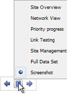 | Floating tab navigator - unticked by default, when ticked this option displays a presentation tab navigator similar to that used in PowerPoint faintly at the bottom left hand corner of each tab. In addition to forward and back arrows for changing tabs sequentially, the central option pops-up a full listing of the tabs in the file, enabling the user to go directly to that tab in the presentation. | Next/Previous buttons - unticked by default, allows you to show Next and Previous arrow buttons at the bottom of each tab as another option for paging through presentations. |
Toolbar settings - Contains settings which control the behaviour of toolbars as the size of the Omniscope window and the display windows within are expanded or reduced.
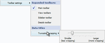 | Expanded Toolbars: Data Titles: |
{new in 2.6 - hold the Control (Ctrl) key down to apply these settings to all tabs, not just the current tab}
Settings > ... groups commands relating to setting options at Tab level, File level, and Application-wide level.
| This Tab: Details - Tooltips - Value colours - Colour ranges - Advanced tab settings -
This File: Images - Links - Web Services - Branding - Advanced file settings -
Application-wide: Language - Window size - Enterprise - {Enterprise editions only} Advanced - |
Help > ... groups commands and links to online resources that can help you make the most of your Omniscope installation.
| Help with this file - opens the file-specific |
The Online help sub-menu contains links to various learning resources:
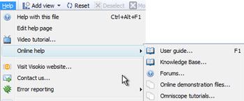 | Online Help sub-menu:
|
The Error reporting sub-menu contains options for sending reports to us automatically, helping to diagnose problems and retrieving error reports that we not able to be send automatically and need to be sent to us as e-mail attachments.
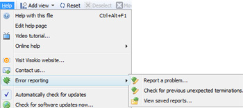 | Report a problem - if your installation is permitted to contact our server at services.visokio.com on port 80, you can automatically file a report that provides us a snapshot of the technical description of you machine and what was happening if an exception (software processing error) is reported while you are working. Please always send these reports, even with queries not resulting from exceptions, since the report provides most of the the technical information we need to respond to you. |
Example problem/error report: No personal information (other than the e-mail address needed to respond to you) and none of your actual data is ever communicated to us in these reports.
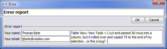
Check for previous unexpected terminations - this is a diagnostic option you will not normally need to use, but we may ask you to use it as part of a troubleshooting sequence.
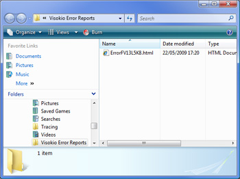 | View saved reports - if an exception occurs while you are offline, or in a location where access to our server at services.visokio.com port 80 has not yet been unblocked, the report will be saved as an HTML file in a location that depends on your operating system. This command will reveal the location of any saved reports. Please always attach these reports to an email addressed to support AT visokio DOT com |
This page lists Main Toolbar command menu items in Omniscope 2.4 which have been re-located in version 2.5. The old 2.4 command menu name/location is shown like this. The new 2.5 command/location is shown like this. Commands whose names/locations have not changed are not listed here.
For the full list of Main Toolbar commands, see the Commands Reference sections for version 2.5 [440]+ or 2.4 and previous [481].
|File [595]|Edit [596] [596]|Tools [597] [597]|Reports [598] [598]|Page [599] [599]|Appearance [600]|Help [601]| |
Omniscope 2.4 File menu
Omniscope 2.4 Edit menu Data menu
Omniscope 2.4 Tools menu Settings menu
Omniscope 2.4 Reports menu Tab menu
Omniscpe 2.4 Page menu Layout menu
Omniscope 2.4 Appearance menu
Omniscope 2.4 Help menu
|
Below is an index to Main Toolbar command menus for version 2.4 and earlier. For information on commands and options related to specific Views and View Toolbars, please consult the Guide to Views. [21] The location of many commands have changed in 2.5 to make finding them clearer and more logically structured. If you're used to Omniscope 2.4, and can't find a command in 2.5, see this guide [572]. See also the full Command Reference for 2.5 [440].
Applies to version 2.4 only; most of these commands are now on the File Menu (2.5) [442]
The File > menu on the Main Toolbar contains commands used to import data into Omniscope, manage .IOK files, and export data from Omniscope in various file formats and as images for printing/pasting into documents. Commands accessible from the File > drop down on the Omniscope Main Toolbar include:
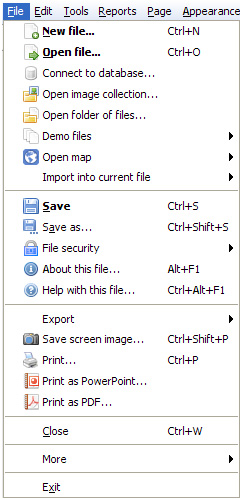 | New - Choosing New creates a new blank table with an initial number of fields (columns) and rows (records) you can specify. The default is 500 rows and 6 columns. If you have an activated Edition, you can set the number of rows and columns to be larger. Once you specify a size, a new blank table will open showing the 3 empty default views; Table View, Pie View and Chart View. In the Table View, right click on column header 'A' and select Tools > Rename field to begin assigning your own names to the fields, then begin entering data as you would for a spreadsheet. Note: You can also administer the naming and data typing of each column from the Edit > Manage Fields menu. Open File - Choosing Open file launches the Open Dataset wizard, which looks like a Windows file browse window, but has some additional features and options on the right side. Navigate your directory structure and find the file you wish to load, be it an existing Omniscope .IOK file, or a data in a supported data file format; Excel .XLS, .CSV (comma separated value) or other delimited text data file formats such as .TSV, .TXT etc. The Open Data Set wizard looks like a Windows file browse dialog:
|
The ![]() Help icon in the upper right of the Open Dataset Wizard [612] displays a format guide [528] for importing spreadsheet files. Always confirm that your spreadsheets conform to this simple layout before trying to open them in Omniscope. For more detail, see Using the Open Dataset wizard. If you encounter problems, see also the Knowledge Base section on importing and exporting data to and from Data Files. [613]
Help icon in the upper right of the Open Dataset Wizard [612] displays a format guide [528] for importing spreadsheet files. Always confirm that your spreadsheets conform to this simple layout before trying to open them in Omniscope. For more detail, see Using the Open Dataset wizard. If you encounter problems, see also the Knowledge Base section on importing and exporting data to and from Data Files. [613]
Connect to database - The Connect to database command launches the Database Connection wizard which guides you through the steps required to import data directly from a relational database table/view instead of an exported data file.
Omniscope uses ODBC or JDBC [614]protocols to access database files. For more detail, consult the Knowledge Base Database Connections [615] section.
Open image collection - Omniscope can be used to inspect and manage collections (folders) of images, for use as embedded image sets in Omniscope, as image folders associated with DataPlayers, or for any purpose where well-organised and documented (large) folders of images must be assembled, inspected, managed and shared with others at any size/resolution. More on using Open Images [42].
Open folder of files - Omniscope can also be used to visualise and navigate collections (folders) of computer files, whether the files are a .PDF document archive on a file server, a collection of podcasts or videos, or the entire contents of your hard disk drive. Omniscope permits you to visualise the relative size and age of the files, sort them based on data modified, etc. If you point Omniscope at a folder containing documents in .PDF format, the documents will display in the Omniscope Web View when selected. More on using Open Folder of files [616].
Demo files - Omniscope installs with a selection of embedded demo files you can use to familiarise yourself with the possibilities inherent in Omniscope. Some of the embedded demo files have associated image sets that can be downloaded when the application is launched. In some cases, you can download the image sets separately and associate and re-size the image set yourself. See Image Sets [617] under the Resources section of our web site.
Open Map - This option is used to add more maps to your installation or import and embed a specific image file for use as a Map View backdrop with a custom co-ordinate system. Freely-downloadable, embedded vector maps from the Visokio Maps Library can be accessed and downloaded at anytime. The Open Maps command displays all the maps which are already stored on your machine (the files are usually located in C:\Program Files\Visokio Common\maps) for use in both Omniscope and Flash DataPlayer .SWF files.
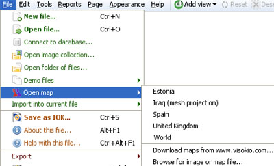
The Open Map command reveals available maps already downloaded, the default world map, the option to download additional standard Visokio maps, and the option to browse for and import/embed an image or customised map file for use as a backdrop with a derived coordinate grid. Recognised map file types for import and embedding include Image (.JPG, .PNG, .GIF, etc. depending on your version of Java), files, plus (Visokio) .MAP, .VEC, and .ILF files. Whether you download a standard map or import a customised map, the next display will be in the Map View [63]. For more information on using geographic coordinate systems with Visokio maps and customising co-ordinate systems for use with imported images such as floor plans or sports fields, consult the Knowledge Base section on Maps & Coordinates [53].
Import into current file - This command reveals a sub-menu containing options for refreshing data from linked sources, administering the data sources linked to a specific file, importing XML query files to recreate record selections sent by others, importing single column lists of references sent by others as .TXT files for matching, merging in (or repeating the merge of) additional columns or rows of data from other .IOK or .XLS/.CSV data files (see using the Merge Data wizard [605]), and importing/refreshing fields from Bloomberg (Professional & Enterprise Editions only, assuming you are running on a Bloomberg-connected PC).
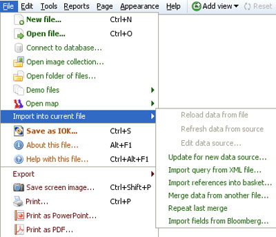
For more detail on the sub-menu commands, see the section on the Import into current file [604] sub-menu.
Save/Save As .IOK - This creates a new Omniscope file based on the existing one you have open. This command uses the same Data Export wizard screens discussed here [532], with the export data file type already set to .IOK, and the same data sub-set and field (column) selection options used when exporting subsets of your data to .XLS or .CSV files. When creating a new version of an .IOK file, you can also choose to save the new .IOK file with additional options:
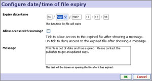
The Save as copy option makes it possible to save the file to another location, without changing the location of the current directory, so you can save an later update to the same base location, for example.
File security - depending on your edition (Professional or Enterprise) allows you to set some of the security options available for the file. For more detail on security options for Omniscope files, see section on file security options [439].
About this file - displays an informational screen giving administrative and licensing details about the open file. For details about your installation of Omniscope, press Ctrl+F1
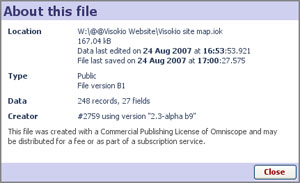
Help with this file - displays the file-specific Help page you can configure for file recipients using the Help > Edit help page wizard. See Help Menu commands [586] for more information and an example.
Note: Publisher-authored Help pages are not currently Report Page-specific.
Export- this command reveals a sub-menu of options for exporting some or all of the data from the current .IOK/.IOM file.
Selecting Export launches the Export files dialog [532] with the export file type already set by default to Excel .XLS workbook files. You can change this to .CSV or other supported data file types.
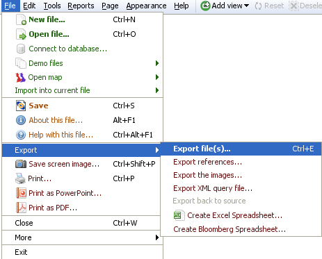
Export references- launches the Export files dialog [532] with the export file type already set to the single column .TXT file format. The wizard allows you to specify the field and records (by universe) from which to generate an exported a list of references.
Export the images- launches the Export files dialog [532] with the export file type already set to a folder of images. The wizard allows you to choose which associated image set you wish to export and to set re-sizing limits on individual picture size to limit the maximum size of the images exported to the folder. Note: Omniscope files make excellent image catalogues. You can view and filter a collection of images, put selected images in the Basket, then export them as a new collection to a folder for re-use.
Export XML query- launches the Export files dialog [532] with the export file type already set to XML Query. This allows you to export your current filter settings (query) or any other named query as a small, portable text file that others (such as database administrators, customers, etc) who have the same Omniscope file can load the query file and instantly focus their display on the exact sub-set of records corresponding to your exported query.
Export back to source- will overwrite the linked data source file (but not a relational database table/view) with corrected/edited data from the Omniscope file.
Warning: if your source data file is a spreadsheet file with formulae, formatting or comments fields, they will be overwritten and lost.
Create Excel spreadsheet- creates a new Excel spreadsheet containing the fields (cxolumns) and data subset you specify. Note that if you want to paste data from Omniscope into an existing Excel spreadsheet, you can also use copy/paste. You must have Excel installed to use these features.
Create Bloomberg spreadsheet- creates a new Excel spreadsheet including imported, automatically refreshing Bloomberg fields i.e. source files that can update in real-time. Professional and Enterprise Editions only. You must have Bloomberg access and Excel installed on your PC to use this feature. For more information, see Working with Bloomberg [404].
Save screen image- Exports the current screen display in a range of image file formats (.JPG, .BMP, .GIF, .PNG, .WBMP) suitable for pasting into other applications. Also provides an option to copy the image directly to the clipboard for re-use.
Print screen- Sends the current screen display to your printer as an image.
Print page- for more detail on Printing, see Printing options [607]
Print as PowerPoint- for more detail on Printing, see Printing options [607]
Print as .PDF- for more detail on Printing, see Printing options [607]
Close- closes the current Omniscope file. Opening a new Omniscope file will automatically close the Omniscope file currently open. You will asked if you want to save your changes first.
Exit- Exits the Omniscope application (but not the Enterprise Edition Scheduler or Generator, which are autonomous applications intended to be run on always-on servers). You will be asked if you want to save if you have made changes to data or view configurations, but neither closing nor exiting will commit changes to Report Pages. The file will next open with the Report Page tabs in red, indicating that you have to either commit the changes or revert to the original configuration of the Report Page.
Applies to version 2.4 only; most of these commands are now on the Data M [443]enu (2.5) [443]
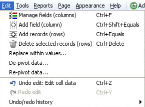 | Manage fields - launches the powerful and useful Manage Fields dialog, from which you can configure nearly every aspect of each field (column) in your data set such as adding, removing, hiding and globally re-ordering fields. Also used to manage/change the data typing for each column (integer number, decimal number, dates and times, text and categories) and to configure and format the way the values are displayed. For more information, see Using Manage Fields. [31] Add field (column) - adds a new, blank field (column) to the dataset. Unless you are in Reports Mode, you will see the new column appear at the far right in the Table View. If you are in Reports Mode, the new column will not be visible until you go to View Tools > Column Options > Columns to show, find the new field at the bottom of the pick list, tick it to reveal the new column and drag it into place in that Table View. This command is also available at the bottom of the Manage Fields dialog. The difference is that if you drag the new column into place using the Manage Fields dialog re-order, it will position the new column globally for all views, not just the Table View (and pop-up Show details table) or a Table View in a Report Page.
|
Add records (rows) - adds a specified number of new records (rows) to the bottom of the data set. This can also be done (with more precision as tgo where the rows are added) from the Table View row header right-click menu.
Delete selected records (rows) - deletes selected rows (can be un-done using Undo edit ...see below)
Replace within values - used to perform global search and replace operations. Choose which fields (columns) you are going to search and replace, then type in exactly the text string to be found, and the string you wish to replace it with.
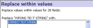
De-pivot/Re-pivot data - Sometimes source data is laid out 'horizontally' when Omniscope would manage it better 'vertically' (e.g. time series), and vice-versa. Sometimes data needs to be exported from Omniscope in an orientation different from that used in Omniscope reports. To avoid the time consuming process of changing the orientation of data from horizontal to vertical (row becomes column) or vertical to horizontal (column becomes row), Omniscope has both a De-pivot and Re-pivot function. Use of these functions is discussed in more detail here [421].
Note: Omniscope does not currently support transposing a data set (exchanging all rows and columns) with or without headers.
Undo/Redo edit - allows you to reverse data editing operations
Undo/Redo history - keeps a history of reversible operations. Operations which can no longer be reversed/re-done are greyed out.
Applies to 2.4 only; most of these options are now on the Settings Menu 2.5 [446]
The Main Toolbar Tools menu and sub-menus group together commands and options for managing data refresh, language settings, 'brushing' or fading of unselected records, display of individual record-level details, links to related content and services outside the file, associating image sets with the file and many advanced configuration options.
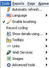 | Automatic refresh - when ticked, displays the Automatic refresh drop-down management menu and Hold button on the right side of the Main Toolbar. |
In addition to using the Details View, there are various options for showing record-level details.
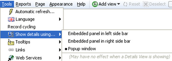
The default (whenever the Details View is not open) is to display details using the pop-up window. If Sidebars are visible, there are options to display details panels at the bottom of either one (but not both) of the Sidebars. For more information, see Viewing Details [23]
Tooltips are temporary text displays that appear whenever you hover your mouse over a marker or other representation of one (or a group of) record(s) in the data set. Using the drop-down pick list, you can select which field values will be displayed whenever Tooltip displays are visible.
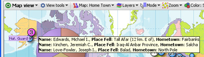
Tooltip displays are Report Page specific. If you are in Reports Mode, the selections you make will be remembered and the selected values will appear in all Tooltip displays on that Reports Page. If you Exit Reports, the Tooltip displays will revert to the defaults you set for the file. Note: Use Tooltips sparingly...selecting too many field values to display will can create large blocks of text values that obscure too much of the open views.
You can also choose to display associated image sets as Tooltips:
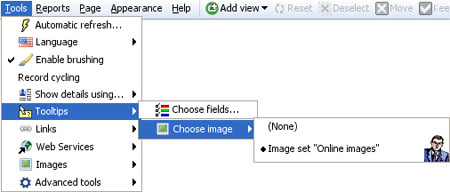
To learn how to associate image sets with your Omniscope files, see Tools > Images below.
Links extend your file users' experience to include content not contained within the Omniscope file itself. By adding links, anyone can integrate related external content (documents, files and web pages) into their Omniscope files, with one-click access via their local network, and the open web.
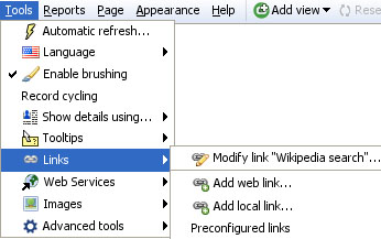
You specify links and make them available for use within your Omniscope file using the Add web link, Add local link and Preconfigured links dialogs. For more information, see Tools > Links [534].
Web Services are data processing services that use Internet standards to post data to a remote server, which usually delivers a response in web page format. Popular examples of Web Services in action include submitting text to a search engine and receiving the results page, or submitting stock tickers to view price charts. (definition of Web Services [619]).
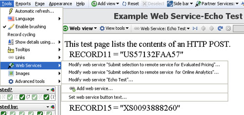
Omniscope is a 'hybrid' web/desktop application that is easy to integrate with Web Services. In addition to the preconfigured free web services (that accept a single value text string input) available on the Links menu, there is also a useful multi-record submit Web Service via HTTP POST available in Omniscope. The Tools > Web Services dialogs permit you to configure and edit Web Services that expect multi-record input to work seamlessly with your Omniscope files. Accepting the defaults under Add web service will configure an 'echo test' service (hosted by Visokio) in which our server repeats back a list of references you have selected in your local Omniscope file. More information on configuring and using web services with Omniscope is available in Tools > Web Services [17]and the Web View [16] subsection on using Web Services [552].
Before you can display images, you must associate one or more folders of images with the .IOK file as a named image set. Preparation for this involves saving a set of images in a single folder with a consistent naming convention, such that the same text values are present in one of the columns of your .IOK file (it may be a column included just to hold the names of the images). It is also possible for Omniscope to display multiple images per record, provided you have entered multiple 'tokenized' values in the image reference cell.
There are 3 ways to display image sets in Omniscope:
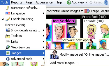
Once you have associated one or more image sets (each with single or multiple images per record) with your file, you can display these images in various views:
For more detail, see Adding Image Sets [620]
Omniscope can be used with any language. You can use existing translations, modify existing translations, or create your own translations files based on those that already exist.
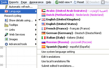
Language selector - choose from the list of available translations
Use system language setting - tick this option to start Omniscope with the language setting specified in the operating system. If a user selects a different language, it will override and untick this setting. That user's installation will open using the preferred language until reset using this command.
Edit translations - opens your local copy of the embedded EditedLanguages.iok translation file. You can make changes to the translations text in this file, being careful to follow the Guidelines in the Translations Guide [465]. When you have finished editing, choose File > Save (not Save As) to save the edited file in its original location. In Tools > Languages, ensure your edited language is selected, then close and re-start Omniscope to see the changes you made via the edited file.
Use local translations file - if you open the embedded EditedLanguages.iok file to make and save changes, this option will be ticked. To revert to showing the default translated text, untick this option and restart Omniscope.
Submit edited translations - if you would like your translations/edits to be included in the default for a given language, or added to the menu as a new language or variant, submit your EditedLanguages.iok file to us using this command.
Additional Tools sub-menus are available from the Advanced Tools menus. Note: Some of these commands are only available in the Enterprise Edition.
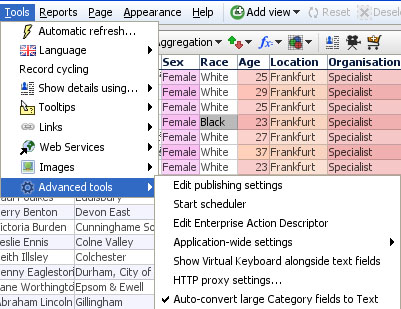
For more detail on these and other Tools > Advanced tools sub-menu commands, see Advanced Tools [621]
The Main Toolbar Tools > Advanced Tools menu and sub-menus include a number of important options, some of which (Edit publishing settings, Start Scheduler, and Edit Enterprise Action Descriptor) are only available in the Enterprise Edition and are discussed in the Enterprise Edition - Advanced Tools section below.
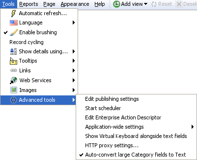 | Show virtual keyboard alongside text fields - tick to enable users to enter text without keyboards HTTP Proxy Settings - useful for activation, updates and automatic bug reporting. For more information, see Proxy Settings [622] in our KnowledgeBase. Autoconvert large Category fields to Text - by default, Omniscope will not treat a Text field (column) containing more than about 200 unique values as a Category field, for performance and other reasons. Sometimes there is some leeway around this depending on the size and composition of your data set, and some views will only display breakdowns by Categories. Unticking this option will allow you to experiment with treating some text fields as very large Categories. |
Warning: There is still a safe upper limit for unique values treated as Categories rather thanText. Trying to convert a field (column) with more than 500 unique values will definitely trigger a warning:
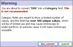
For more information on data typing and converting text fields to categories, see Edit > Manage Fields [31].
The application-wide settings sub-menu is used to configure various aspects of your Omniscope installation that apply to all files you open.
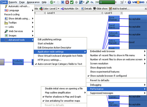
Embedded web browser - allows you to change the installed browser underlying the Web View and Outside browser (see below). Current options include Internet Explorer and Firefox/Mozilla.
Number of recent files to show in file menu - allows you to specify the number of recently-opened files to show at the bottom of the File menu.
Number of recent files to show on welcome screen - allows you to specify the number of recently-opened files to show under Recent files heading on the Welcome screen {version 2.3+}.
Screen resolution - Used to tell Omniscope the type of display screen the file will be used on (Handheld, Projector, Desktop or Kiosk/TV), so that layout, font size etc. can be optimised. This is the same as the display setting on upper right of the the Welcome screen {version 2.3+}. This is not the same as the option to change only the resolution displayed, which does not affect Omniscope's choice of layout, font size, etc. See also the command Appearance > Resize window to [569]: which changes only the resolution displayed.
Show diagnosis tools - this option reveals some additional error reporting options, for example a menu item to report errors on loading images from image sets. We may ask you to enable this to help with troubleshooting.
Show experimental features - every version of Omniscope contains some experimental features which are still under development.Tick this option if you want to reveal (in violet font) and test these features.
Show outside browser if configured... the Outside browser is an Omniscope web browser view which can opens alongside the Welcome Screen before any specific Omniscope file is opened. It is different from Web Views, which are configured within each file to open pointing at pre-defined links/web services as required. The Outside browser feature is used to provide a group of users the ability to browse and select from a library of Omniscope and other data files displayed on a (usually permissioned) web page. For more information, see Using the Outside Browser [623].
Revert to defaults - resets all Application-wide settings menu options to the default settings.
Debugging - used to create log files that record each event in various processes. We may ask you to tick some or all of these in order to generate a log file we can review to help us troubleshoot problems.
Disable initial views on opening a file - this setting enables you to explicitly control, one-by-one, the views that open with your data. It is used to recover files whose initial opening configuration becomes unusable for some reason, or where opening very large files on machines with limited RAM that require the utmost conservation of memory. Warning: If you leave this setting ticked, all files will open with no views showing....use only when dealing with specific circumstances.
Map outline simplification - reveals a sub-menu which allows you to adjust the resource demands associated with drawing and zooming/up-dating maps.
Marker shadows in Map and Graph Views - unticking this will improve performance in some files with very large numbers of markers visible in the Map or Graph Views.
Use anti-aliasing for smoother maps - unticking this will improve performance in some files with extensive use of maps
Reset to defaults - resets performance options to the default settings
The Enterprise Edition contains advanced automation, and file security revenue protection features useful in commercial data publishing:
Edit publishing settings - {Enterprise Edition only} this dialog is used to set the publisher identification text and links that will appear whenever a file recipient clicks on File > About on a file produced with this installation.
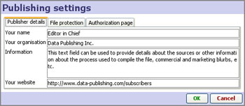 | 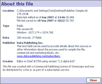 |
Edit publishing settings: file protection options - {Enterprise Edition only}
Protected- used to prevent data editing, export and copying (including copy-and-paste copying). Other options to time-limit or password-protect files are available from the File > Export or Save as [544] dialog.
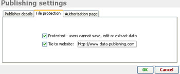
Tie to website - {Enterprise Edition only} enables domain locking, a powerful and effective revenue protection feature. Omniscope .IOK files are free-standing and easily transferred by e-mail, posting/downloading from blogs and websites, etc. Commercial publishers can use this domain-locking feature to require that anyone trying to open their files must be logged in to a specific web site. If the file recipient is not logged in, the .IOK file containing the data will not open, and will display a notice to that effect:
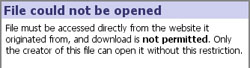
Start Scheduler - {Enterprise only} the Scheduler is Visokio application separate from Omniscope used to automate the refresh, import, merge and publishing/distribution of data files by defining a set of actions performed repeatedly on a specified time cycle. For more information, see Using the Scheduler [624].
Edit Enterprise Action Descriptor - {Enterprise only} the Scheduler uses Enterprise Actions Descriptors XML files, which you can configure using an Enterprise Edition user interface, or manually, based on a exported example specification. [625] Examples of actions which can be automated include:
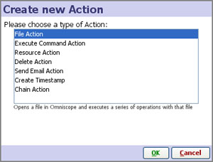
For more detail, see Creating and Editing XML Actions [626]
Applies to verson 2.4 only; most of these commands are now accessed from the Tab Menu 2.5 [444] or the "+" icon to the right of the final tab.
The Main Toolbar Reports menu provides access to all the commands used to create and administer Report Pages configured in the file. If no Report Pages are yet configured, you will see only the Create Page heading on the menu. If Omniscope is currently displaying a combination of views, queries, variable settings, etc. that you would like to make persistent, you should choose to create a Reports Page. Professional and Enterprise Editions can create any number of persistent, tabbed Report Pages, with sectioning and other advanced tab options.
| Create page from current Omniscope configuration. You will enter Reports Mode and all your current settings will be copied to create a new Reports Page. In Reports Mode, any further changes you make will apply only to the open Report Page, and all subsequent changes must be Committed to become persistent (see below). |
The commands below are also accessible from the Reports Navigator, which appears in the lower right-hand part of the screen when the file is in Reports Mode. These commands are more fully documented below in the Reports Navigator section.
Administer all pages - if you already have Reports Pages configured in your file, you can manage modifications to all pages, or delete them all using these commands.
Navigation: Start ; ...Go to Page - if you already have Reports Pages configured in the file, these commands allow you the access any Page, from the start or from a drop-down menu that appears on the right of the Go to Page command.
Show report tabs - this option displays a tab for each Report Page across the top of the Main Toolbar, even if you are also displaying buttons in the Side Bar Reports Panel.
To create a Report Page from the current display in Omniscope, or as a text or image slide/imported PowerPoint slide, use Reports > Create Page from the Main Toolbar Reports menu. If you have revealed the Sidebar Reports Panel, you can also click New to access the Create New Page wizard:
 | Page name: this name appears on a report tab at the top of the display, or a button on the Side Bar Reports panel if you provide access to Report Pages there. You can change this name at any time on the tab or in the Reports panel. It is best to keep the page name relatively short, as you can use Title and Annotation fields below to convey more detail. |
Annotation: explanatory text to focus the readers' attention on specific aspects or actions. You can edit this at any time by double-clicking on the annotation text field.
Header/Background Image - adds images to each Report Page; Header images display at the top of the page, Background images can be faded and display in views that otherwise display blank backgrounds. For more information on fading background images, see Page menu commands. [567]
Apply default report layout: If you leave this box ticked, Omniscope will hide the View Toolbars and increase the margins around the views for a cleaner display. If you wish to preserve the existing settings, untick this box.
Once configured and named, each pre-defined, persistent Report Page appears anytime the user clicks on the top report tab, or the button next to the Report Page name in the Side Bar Reports panel, or uses the Report Navigator menu, which appears faintly in the bottom left corner of the display in Reports Mode.
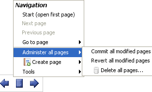 | Start; Next; Previous; Go to page...used to cycle through the Reports Pages already configured in the file. |
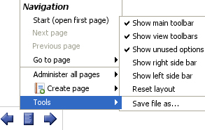 | Show/Hide main toolbar- when unticked, the Main Toolbar is not visible unless the user hovers the mouse near the top of the display. |
Reset layout - returns the page layout to the defaults, such as the Main Toolbar displayed, Report Tabs displayed, etc.
Save file as... saves the open file with a new name and/or settings and options, using the Export file as .IOK/.IOM [544]dialog
From the optional Sidebar Reports panel, you can group your Reports into sections, as shown in this example file [627]. To create a section name, choose Create New > Section at the bottom of the Sidebar Reports panel. Rename or delete sections using the black triangle drop down. Drag and drop to reorder reports in sections.
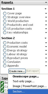
You can also mix query-only and view-only reports. To create such query-only or view-only report items, choose Create new Omniscope page from the New... button in the Reports panel, and select either Query state or Views and layout configuration.
This example file [627] illustrates navigating a set of query-only reports, grouped under a section name in the Side Bar Reports panel, and a set of view-only reports configurations, also grouped independently. This allows you to configure a set of different view configurations (by task, or form of analysis, such as 3 Web Views, or a Graph and a Web View, or 2 Pie Views) and an independent set of queries (such as last week's, or last month's trades, or erroneous trades) enabling users to navigate any combination independently. For example, a user might open Query A then Views X. They can then choose to either change to a Query B while keeping Views X displayed, or Views Y while keeping Query A displayed.
Note: the buttons in the Sidebar Reports Panel only highlight the last report item opened. If you open Query A then Views X, you will see only Views X selected in the Reports Panel. The view configuration from Views X will be showing and the filters will continue to represent Query A correctly. But because only Views X is actually selected, manipulating the query will not affect Query A.
Applies to version 2.4 only; most of these options are now on the Layout Menu 2.5 [25]
The Main Toolbar Page menu commands provide many options useful for creating more informative displays and Reports Pages. The commands on this menu can be used to configure many aspects of the current display. If you make changes to the current view using Page menu commands, then close and save the file, it will next open with those changes preserved in the current display, even if the display is not configured as a Report Page.
Page menu commands can be used to:
| Reset layout - removes any changes which have been made to the margins and other layout settings. If no changes have been made, the command is greyed out.
|
You can also tick/untick the options to Show/Hide the Main Toolbar and the View Toolbars for all views on the page. View Toolbars can usually be hidden if the users of the page are not expected to need access to the options available on them. Even when hidden, the Main Toolbar comes back into view whenever the user hovers the mouse near the top of the display.
Page menu commands apply to each Report Page individually, and any changes must be Committed to become a persistent change, or Reverted to return the Report Page to its default configuration/layout. For options covering aspects of the look and feel of Report Pages that apply to more then one page, see the Appearance [628] command menu.
Title and annotation text can be styled by choosing the font, the font size and face, as well as the horizontal alignment and text colour:
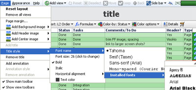
Background images can be faded so that they interfere less with other aspects of the display. Use the Fading slider to adjust the intensity of the image, from weak (very faded) to strong (barely faded).
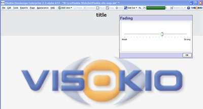
Background image options also include 3 Crop style options for fitting background images of any size/aspect ratio to the display:
Header images are not intended to be faded and/or resized, as they are generally logos whose aspect ratios and legibility must be preserved. If you use a tall header image, it will increase the size of the margin at the top and reduce the display space usable for views.
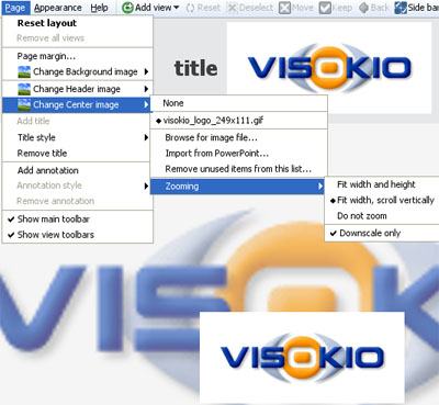
Centre images can be made from PowerPoint slides or other large screenshots. They are not intended to be faded, but do have zooming options and a control to stop the picture clarity from being reduced by up-scaling.
Applies to version 2.4 only; most of these options are available on the Settings menu 2.5 [446]
Omniscope files can be used not only to assemble, check, analyse and transform data, but also to distribute as interactive final reports and presentations for various audiences; senior management, customers, partners, friends...anyone with an Omniscope free Viewer or better. The Appearance menu commands enable you to change almost everything about the Omniscope display to conform with your desired look and feel and provide the simplest file opening experience for recipients of your files.
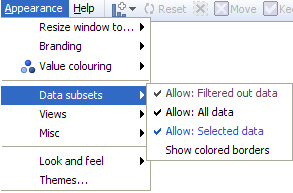
Allows you to resize the Omniscope display to preview how your Omniscope reports and presentations will look at various screen sizes ranging from SXGA (1280x1024 pixels) down to QVGA (320x240 pixels).
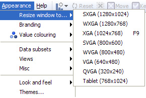
The Resize window to option only changes the size of the display. You can also adapt the default spacing of layouts, margins, font type and size, etc. to various screen types (Handheld, Projector/Laptop, Desktop and Kiosk/TV) using the Resolution option on the Welcome screen, or from the Main Toolbar Tools > Advanced Tools > Application-wide settings > Screen resolution.
Omniscope is a data file publishing system that supports a wide range of branding and corporate identity options. This includes advertising placement options for data publishing business models supported by advertising revenue.
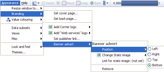
Set cover page; back page - these pages are informational displays (not interactive Reports Pages)
Clicking on the option to configure a Cover or Back informational page launches a Set ... Page dialog that accepts 5 inputs from you. The dialog to create the Back informational page is very similar to the Cover page example shown below:
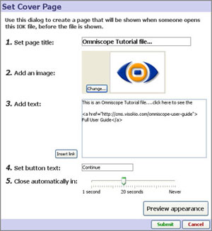 | 1. Set page title: enter text to display at the top of the page 2. Add an image: select an image to display (.JPG,.GIF,.BMP,.PNG depending on Java version) 3. Add text: add the text you wish to display, with hard returns to wrap the text evenly and keep the box size from becoming too wide. Basic HTML tags can be used to style the text Insert link: generates the full HTML to make a link you enter live. 4. Set button text: changes the text displayed in the button from 'Continue' to whatever you prefer 5. Close automatically in: sets the time delay to display the page (not used for the Help Page) |
When you are happy with your information page, click Submit to save the configuration and make the page active.
Add corner logo - allows you to replace the small Visokio logo in the upper right hand corner with a logo of your own. For best results, use a logo image about 19 pixels high. If you change the logo, the link associated with it will be changed to the URL you have entered under Set publisher link (see below).
Add Web Services logo - allows you add a logo to the Web Services menu tab on the Main Toolbar. For more information, see Configuring Web Services [550]
Set publisher link - allows you to enter the address of a web page (URL) that will be displayed as an active link in the File > About this file notice for all files produced with your installation. If you have substituted your own logo for the Visokio corner logo, clicking on your corner logo will also take the user to this URL.
Banner adverts - Omniscope supports the display of banner adverts with live links to the advertiser on each page. The adverts can be positioned at the top, right, left or bottom of the display, and do not affect placement of header images, titles, etc. In general, rectangular images look best, such as typical full-width banner ads. Note: Server-based deployment, Flash .SWF display, embedding animated .GIF images and Report Page specific adverts are not currently supported, but this may change in future versions. For more information and examples, see Advertising Options [629].
Omniscope makes extensive use of colouring by values to help you and the users of your files visualise the relationships, relative magnitudes and overall meaning in your data sets. The Appearance > Value colouring sub-menu contains options to change the way ranges of values within fields (columns) are coloured. It also has options to assign colours to specific values in fields automatically and control the colour palette Omniscope uses to assign initial colours to Category values. You can override colour assignments for specific values and range endpoints at any time using the colour selectors available in Edit > Manage Fields > Configure >Field Options > Change value order, colours and shapes.
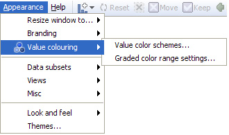
Value colour schemes - clicking launches a dialog that enables you to manage various aspects of colouring values:
Presets: a number of pre-configured combinations of settings are available, including 'Corporate Blue', 'Subdued' and 'Monochrome' colouring schemes. If you make changes to the defaults to create your own scheme, you can name it and save it for future use with specific files. To return to the default 'Classic' Presets, click on Revert to defaults.
Category fields:
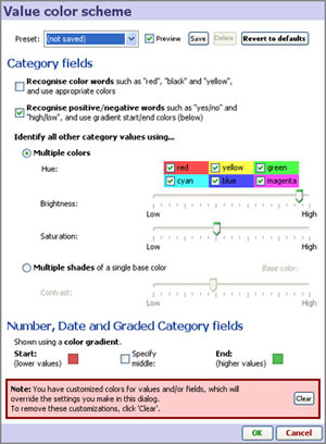 | Recognise colour & positive/negative words- when ticked, these options automatically assign pre-defined colours to recognised text values, such as 'red' or 'green' or 'yes' or 'no'. |
Number, Date and Graded Category fields - fields (columns) consisting of defined ranges of values, such as Number, Date & Time and Graded Category fields, are coloured according to a spectrum calculated based on the range between the lowest and highest values and the start (lowest) and end (highest) colour specified here. The default or 'Classic' scheme uses a range from red (lower values) to green (higher values). You can change the default here by clicking on the Start or End colours, and optionally specify a middle value to extend the colouring more or less depending on the middle colour chosen. At any time, you can change the colouring scheme applied to a specific field (column) using Edit > Manage Fields > Configure > Field options > Change value order, colours and shapes.
Note: If you do override the settings made in this dialog for one or more fields (columns), you can clear all of your customised settings using the Clear button shown above.
Graded colour ranges - this dialog determines default behaviour in colouring ranges for Number and Date & Time fields (columns).
Middle colour position: - by default, Omniscope assigns the middle colour of a range to the middle value in the field. This works well for relatively uniform distributions of values. However, if some very high or low values are present in the field, the result can 'compress' the colouring scheme such that there is not enough difference in colouring for most of the records.
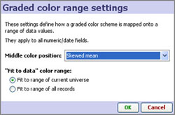
If many of your columns contain such 'skewed' distributions of values, you may want to set the default behaviour to assign the middle colour to the mean (average value), or for even more skewed distributions, to the skewed mean. If only a few fields (columns) are skewed, you may want to set the treatment of the skewed fields individually using Edit > Manage Fields > Field options > Change value colouring.
Fit to data colour range - Omniscope manages colour ranges in two modes; a filtering-neutral mode, which assigns and displays colours based on the full range of values in the field (column), and a dynamic filtering re-colouring mode, which re-calculates the range and re-assigns colours based on the range of values present in the universe being displayed. The default is the dynamic re-colouring mode, Fit range to current universe, but you can change the default setting here by selecting Fit to range of all records instead.
Omniscope selection, filtering and basket management functions assign every record in the data set to multiple data universes. By default, every view can be opened on any of the 5 universes, and each view indicates the target universe being displayed by the colour of the corner 'eye-con' and the view selection menu.
Allow OUT; ALL; SELECTION; BASKET - depending on the file and target users, you may want to simplify the menus and options by preventing views being opened on certain universes, such as the OUT or ALL universes. If these universes are not being used in Report Pages and could confuse novice users, you can prevent viewing them by removing them from the View Chooser. You can turn off access to all universes other than the IN universe by unticking them here.
Note: Users can re-enable access to universes on this menu, but not save changed versions of the file, provided you ticked the Prevent data edit/export option when you last saved the Omniscope file
Show coloured borders- this option provides for more visual impact by displaying a coloured border around each view indicating the target universe for the view.
Depending on the file and target users, you may want to simplify the display options by removing the Add View option from the Main Toolbar, or by removing certain views from the View Chooser. This could be because the view(s) are not useful, or because the size/configuration of the file makes some views slow relative to the usefulness of the view.

Note: Motivated users of the file can still access this menu and re-enable the view(s), so these are just menu simplification options rather than a short-cut to avoid configuring all views as meaningfully for your data as possible. However, provided you ticked the Prevent data edit/export option when you last saved the .IOK/.IOM file, any user that re-enables or otherwise changes the file settings in the Appearance menu will not be able to save or forward a persistent version of their changed .IOK/.IOM file.
Omniscope is designed to be used for analysis, but also for distribution as final reports, for giving live presentations and for printing as static PowerPoint slides or Adobe Acrobat .PDF documents. Depending on the immediate use you have for the file, you may wish to modify certain aspects of the display:
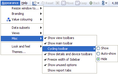
Show/hide view toolbars - untick this option to hide the View Toolbars, making the display appear more like a final report/presentation
Show/hide main toolbar - untick to hide the Main Toolbar across the top (it will always re-appear when the mouse hovers near the top of the display)
Freeze width of Side Bar(s) - untick this option to allow users to narrow or widen the Side Bars (Report Page-specific)
Show unused options - untick to simplify menus by removing references to options not used in the file.
Show report tabs - untick to hide report tabs at the top, under the Main Toolbar.
In addition to defining colouring schemes for value ranges, you can also manage the overall aesthetics of your file using the options available on the Appearance > Look and Feel sub-menu. The options available on this sub-menu are used to define Themes, combinations of settings you can use to, for example, mute the colouring application-wide to achieve a more corporate look. The best way to see the differences these settings can make is to try applying the pre-configured Themes (see below), then opening the Look and Feel dialog and noting the settings used. Note: Look and Feel menu options are Report Page-specific. To apply the same settings to all the Report Pages in your file, choose Apply these settings to all pages.
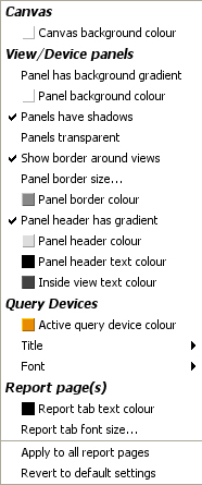 | Canvas: Canvas background colour - sets the colour of the background displayed when no view is open, in the margins, and behind the title and annotation text. Query Devices settings: (see below) Report Page(s) settings: (see below) |
Query Devices settings: (displayed on the Sidebars)
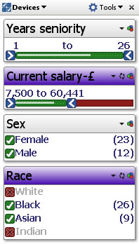 | Active query device colour - changes the colour indicating that a filter/query device is active from the default dark orange to any other colour (purple in the example left) |
Report Page(s) settings: Tabs
Report tab text colour - sets the colour of Report Page tab text
Report tab font size - sets the size of the Report Page tab text
![]()
Themes are combinations of settings of options for Look & Feel. A list of pre-defined Themes come with the application. You can modify these Themes, or create your own, and save your modified settings as a new Theme with a name you assign. Your Theme(s) will be saved in your program folder and will be available for use in all files you prepare with your installation. There is the option to apply the Theme to all Report Pages.
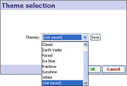
Note: From version 2.5 onwards, Themes are referred to as Styles
Applies to version 2.4 only; most of these commands are now on the Help menu 2.5 [447]
The Main Toolbar Help menu contains links to a wide range of learning and support options:
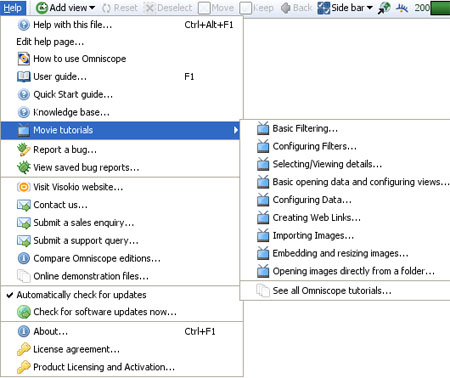
Help with this file- launches the file-specific Help page display you can create to explain the finer points of your file to users. You create this Help page for each file using the Help > Edit help page command below.
Note: Help with this file screens are not Report Page specific...use Annotations and Field Notes instead.
Edit help page - opens the Set Help Page dialog to compose your help page
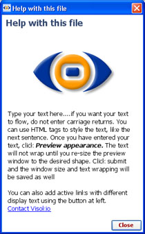 | 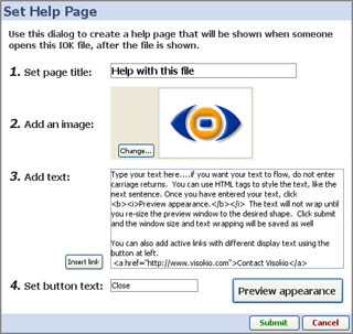 |
How to use Omniscope - launches the embedded, interactive, tabbed tutorial file illustrating the major features of Omniscope.
User Guide - links to this Omniscope User Guide [592]
Quick Start guide - links to the one-page introduction [384] contained in this User Guide
Movie tutorials - links to various Flash screencasts illustrating common tasks in Omniscope.
Report a bug - if Omniscope displays an error message (throws an exception), or if you see something you think is a bug, please use this form to tell us about it.
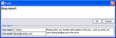
Try to give us as many details as you can regarding what you were doing at the time. This will help us try to reproduce the problem. If the file does not respond, send us the file if you can. If your machine hangs, there is a Hang Diagnosis procedure [630].
View saved bug reports - If you are offline when filing bug reports, Omniscope will save them for review and forwarding to us via e-mail.
Visit Visokio website - this links to our main site homepage at www.visokio.com [591]
Contact us - links to our contact page [86]
Submit a sales enquiry - links to our contact page [86] for license sales
Submit a support query - links to our contact page [86]for support
Compare Omniscope Editions - links to our comparison chart [479] summarising differentiating features of the various editions of Omniscope.
Online Demonstration files - links to our main demos page [631], which features more and larger demos than those embedded in the application. Embedded demos are accessible from the Main Toolbar under Files > Demo files and from the opening screen Demos section.
Automatically check for updates - tick this option if you want Omniscope to check for a newer version every time you start the application
Check for updates now - confirms that you have the latest version installed
About - very useful display of your edition/version number, whether or not you are licensed for Commercial Publishing, your license key number (keep a copy in a safe place) and the version of Java that Omniscope is using (there may be more than one version of Java on your machine).
License agreement - links to our licensing page [632]with full text copies of our licensing agreements.
Product licensing and activation - this menu is used to convert a free Viewer to an activated Edition, and to deactivate an activated installation prior to re-building the machine or moving the key to another machine (you may do this a maximum of 3 times). It is also advisable to periodically Refresh your activation after installing a newer version over an older one. For more detail see the Activation and Refresh [633].
Omniscope can connect to and import data from any relational database that supports common protocols like ODBC and JDBC. The Database Connection wizard guides you through the process of connecting and importing your data, and saving it as a new Omniscope file. Your file will remember its source(s), and on refresh re-execute the embedded SQL statement to re-generate the reporting view/table and repeat any subsequent merges with other files either on opening, or on demand.
The Omniscope Database Connection wizard lets you define a connection and pass any standard SQL expression that results in a single 'flat' table. If you do not have authorisation to execute SQL statements, or don't know the SQL required to generate the table you want, your Database Administrator may have to create the connection in the wizard and/or create the appropriate reporting view(s).
Some organisations also have additional high-performance analytical and reporting databases that pre-prepare data for reports by performing joins, aggregations, sorts and scans on data assembled from multiple transactional databases. In general, Omniscope interacts with 'business intelligence' analytical databases in exactly the same way as transactional database views/tables. For more technical information, see the Database Connections [474] section of the KnowledgeBase.
Clicking on File > Connect to database launches the Database Connection wizard. The wizard guides you through a six-step process for defining a linked data source from a relational database view/table. You will need to know the type of database and its connection details. Using the Database Connection wizard, you enter the connection details for your database and choose which database table or reporting view you wish to retrieve data from. By default, this will create a persistent linked data source relationship between this database table/view and the Omniscope file.
 | 1. Connection type: Select the type of connection you are creating from the options currently available.
ODBC - use this option to connect to defined data sources, like MS Access. Can also be used to connect to spreadsheets for testing.
JDBC - use with databases other than MS SQL Server & Oracle if you have the JDBC driver installed.
MS SQL Server - use this option with MS SQL Server 2000. If you have 2005 or 2008 use the generic JDBC option.
Oracle - use this option with all versions of Oracle databases
Detailed examples of each type of connection are available in our KnowledgeBase. [634] |
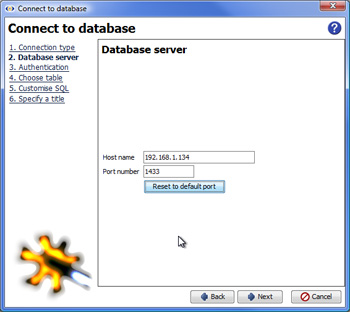 | 2. Database Server (ODBC configuration): Assuming you chose the most common ODBC connection type , you will be asked for a name, or if you are rolling out auto-refresh from the database to a large number of desktops, a DNS-less connection string [635]may be preferable. For examples of various connection types and an exlanation of easy-administration connection strings, see the KnowledgeBase. [634] |
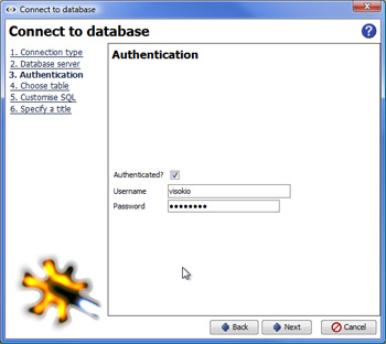 | 3. Authentication: if access to the database view/table is authenticated, tick the box and supply the Username and Password combination to be used whenever the file is refreshed. |
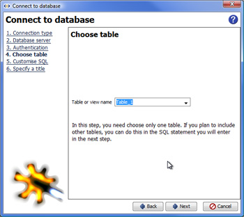 | 4. Choose Table: assuming the comprehensive data set (database reporting view) has already been created as an ODBC-required single table, enter the name here: |
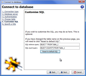 | 5. Customise SQL: If you know SQL and your database, you can modify the default statement and your statement will be saved and re-evaluated each time the file is refreshed. If there is a need to exclude some records in the linked database view/table from the Omniscope file, queries can be added to the connection. These can be refined/edited at any time using Data > Edit source. If you have several related queries, you may want to save each SQL statement in a text file and paste them in with minor variations. Note: If you want o modify the SQL statement programatically using Enterprise XML actions for automated refresh and distribution using the Scheduler watch folder [636], please contact us. |
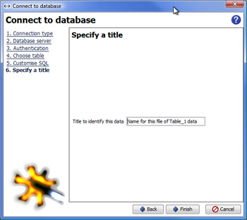 | 6. Specify a title: Choose a name for this linked relational database source, ideally a name that communicates something about the underlying SQL queries (if any) being used. |
Sometimes source data is laid out 'horizontally' in rows when Omniscope would manage it better 'vertically' in columns. Sometimes data needs to be exported from Omniscope in a layout/orientation different from that used in the Omniscope file. To avoid the time-consuming process of changing the orientation of data from horizontal to vertical (row becomes column) or vertical to horizontal (column becomes row), the Omniscope Edit menu has both a De-pivot data and Re-pivot data function.
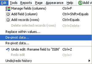
Data tables containing repeated observations of values sometimes place each set of observations in a column, such as the example of daily bond yields by ISIN identifier below. This 'horizontal' layout with the dates of each observation in a separate column is not useful for time series analysis in Omniscope, so we use the Edit > De-pivot data wizard to change the layout/orientation of the data set:
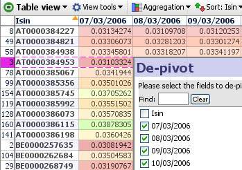
In this case, the ISIN identifier is already in a single column, so we do not need to create another column. We therefore untick this column from the list of columns to be De-pivoted as shown above.
In the new data layout, we want all the dates of reported yields/prices to be in one column, which we can re-name 'Date' or similar. Next to the new 'Date' column (the pivot series values), for each ISIN we want the observed Yield/Price for that day (the pivot cell values), which we can rename accordingly:
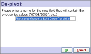
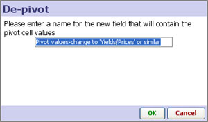
Given the information above, Omniscope will automatically change the data layout/orientation accordingly, with the ISIN reference duplicated for each date, and the column names changed to those you specified. Note: do not worry about the 'vertical' duplication of the ISIN values. This duplication is only visible in the Table View and does not appear in the reports and charts
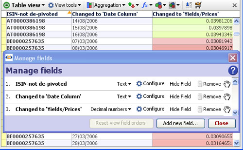
With the data now in 'vertical' Omniscope layout, we can use the Graph and other views to display the time series:
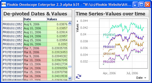
Sometimes you may need to do the reverse of De-pivoting, i.e. converting a single column into many different columns by unique values. For example, you may need to export a data set in spreadsheet format with a layout/ data orientation different from that used in your Omniscope reporting file. The Edit menu also contains a Re-pivot data function which performs these changes in data layout or orientation automatically. In the example below, we are going to convert this data set from the 'vertical' layout with the dates all in one column, to a 'horizontal' layout with a column for each date and the observations under each date.
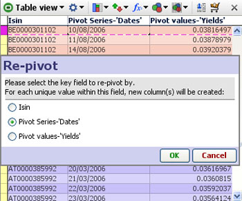
We want to keep the ISIN column as a column, so we select Dates as the pivot series as shown above, then we select Yields as the value fields to be arranged under the new date columns as shown below:
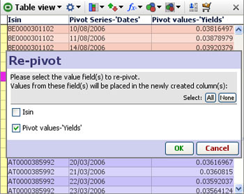
The result of the Re-pivot is a typical 'horizontal' data layout/orientation:
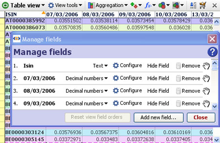
To merge data from another file into your own Omniscope file, you must have at least one column in your data matching one of the columns in the external merge file(s). For example, to use a data file such as our By Countries merge files, you must have at least one column in your data that has the names of countries, or their ISO codes, or other standard identifiers.
Note: Sample IOK merge files containing decimal geographic coordinates for countries and major cities, plus examples of other useful reference data available to merge into your data files are available here [60].
To open the Merge Data wizard, click Main Toolbar: Data > Merge and the Merge Data wizard will appear:
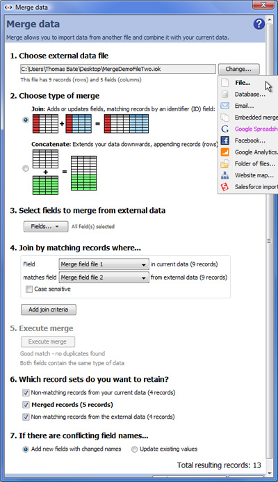 | 1. Choose external data file - point to the external merge file containing the fields (columns) you wish to add to your data set. You will need to specify what type of data source you will be merging. 2. Choose type of merge - you have a choice of two types of merge, Join or Concatenate. To add new fields (columns) to your data from a separate Merge File, choose Join. To add files with duplicate column names together, for example to combine multiple regional report files to form a single global report, choose Concatenate. (see examples below) IMPORTANT: fields being used for merge criteria may have duplicate values in one file, but not in both files. Before performing a merge, always check the uniqueness of the fields (see below) If you chose Concatenate, all the Join options will be greyed out. Scroll to the bottom and... 5. Execute Merge - for Joins, the wizard provides feedback on the matching process, reporting records in your current data not matching any incoming merge file records, exact matches and external records that do match any records in your starting file. Press [Execute merge] |
Note: If you use Date and Time fields as Join criteria, the names of the fields (columns) can be different but be sure that the format of the data in both fields is exactly the same.
SUGGESTION: Before using a field (column) as a join criteria or matching field, it is good practise to check whether the values in the matching fields in both your starting file and the incoming merge file are unique (using Table View: View Tools > Tools > Select duplicate records). If both columns are unique, for a Join the number of merged records will be the same as the number of matching records, plus any non-matching records if you choose to keep them. If your starting file's matching field has duplicate records (such as multiple addresses with the same post code), Omniscope will warn you that permutations (additional records) will be created in the resulting merged file so that all address records receive their map coordinates. If you attempt to merge two files, both of which have duplicate values in the matching fields, try to specify as many additional join criteria as you can so as to minimise the number of permutations created.
7. If there are conflicting field names...- duplicate column names are normal for Concatenations, but before accepting the results of a Join, you must choose how to treat duplicate column names, i.e fields with exactly the same name in both files. There are two options:
Add new fields with changed names - in the event of duplicate column names, Omniscope will notify you that new columns are being added and modify the names of duplicated columns by adding a (2). See example below.
Update existing values - if you choose this options all values in columns of the starting file will be overwritten by the values in the incoming file if the column names are exactly the same. If you choose this option, ensure that the data in the incoming file always supersedes the data in the starting file. See example below:
To finalise the merge, Click OK, Apply Merge to modify your file by adding in the corresponding column values from the Merge File.
WARNING: Before starting to merge, it is good practise to protect your source files from accidental overwriting by saving then with the 'Warn on save' options ticked. If you click File > Save (or Ctrl+S) after merging, your original data file will be overwritten with the merged file. If you want to preserve your original data file (recommended) be sure to use File > Save As to save the merged file as a new file with a different name.
Demo files used in this section are available for download here:![]() MergeDemoOne [637],
MergeDemoOne [637], ![]() MergeDemoTwo [638],
MergeDemoTwo [638], ![]() Concatenated [639],
Concatenated [639], ![]() JoinedAddNew [640],
JoinedAddNew [640], ![]() JoinedOverwritten
JoinedOverwritten
[641]
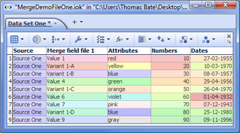 [637] [637] | 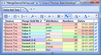 [638] [638] |
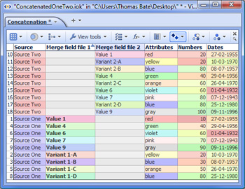 [639] [639] | Concatenating the example data files aligns all the values in columns with identical names, but not in columns with different names. Notice how in the combined file, the values in Merge field file 1 are in a different column from the values in Merge field file 2. If these values were in fact comparable, you could use cut-and-paste to move the values from the second column to the first a delete the second column. |
| Joining the data files above adding new columns for duplicate field names results in 4 new columns being added. |
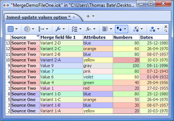 [641] [641] | Joining the data files above updating the values in the current file (Source One) with the values in the incoming or external file (Source Two) overwriting the values in the current file. |
Omniscope is capable of supporting potentially all the languages of the world. To see the available languages, go to the Settings > Language menu, also shown on the Welcome screen. Some of the languages may not yet be completely edited for new features and may have auto-translated phrases.You can easily switch languages without reinstalling Omniscope, although restarting Omniscope is necessary.
Note: only verified translations more than 90% human-edited will be shown. To see other unverified or incomplete languages containing auto-translations yet to be edited, you must first enable experimental features from Settings > Advanced (Application Wide) > Show experimental features.
Anyone can contribute new and improved translations. You can make minor corrections, create country-specific language variants and use your local translation file, or add an entirely new language, using only Omniscope. You can do this privately or you can send your translations/edits back to Visokio for inclusion.
We offer Translators free 3-month Omniscope Desktop license keys, extendable by another 3 months following successful translation of the current release candidate. If you would like to participate in our Translators/Editors program, please contact us. [86]
(Please scroll down to see some example use cases/guidelines.)
For example, you are correcting the Spanish in the "Es" field, which might have been machine-translated. Edit the cells in the Es column directly, making sure you preserve text inside {curly} brackets and html tags inside <angular> brackets.
Make sure the status column is showing. For our example, this would be called "Es status". For each cell you correct, remove the "Auto-generated" text from the status column, if it exists. If there are any comments you wish to add, put them in the status field.
Case B: Translating a language for the first time
You need to create 2 columns:
For example, we have already translated into Spanish (Spain), and you want to translate local variations for Mexican Spanish.
In this case the default language column (named using the 2-character language code) already exists (e.g. "es" for spanish). Following the above example, to add translations for Mexican Spanish you would create the column "es_MX" and translate just those phrases that are different in Mexico. Where the default Spanish translation is sufficient the cell can be left blank.
There is a Forum section where you can query the meaning/clarity of the terms you find in Omniscope:
http://forums.visokio.com/categories/translation [644]
You must be registered on the Forum and logged in to see these discussions.
Links:
[1] http://kb.visokio.com/video-tutorials
[2] http://kb.visokio.com/view-toolbar
[3] http://kb.visokio.com/table-view
[4] http://kb.visokio.com/chart-view
[5] http://kb.visokio.com/pie-view
[6] http://kb.visokio.com/bar-view
[7] http://kb.visokio.com/graph-view
[8] http://kb.visokio.com/display-time-series
[9] http://kb.visokio.com/tile-view
[10] http://kb.visokio.com/pivot-view
[11] http://kb.visokio.com/network-view
[12] http://kb.visokio.com/portal-view
[13] http://kb.visokio.com/map-view
[14] http://kb.visokio.com/connect-markers
[15] http://kb.visokio.com/venn-view
[16] http://kb.visokio.com/web-view
[17] http://kb.visokio.com/web-services
[18] http://kb.visokio.com/content-view
[19] http://kb.visokio.com/dial-view
[20] http://kb.visokio.com/details-view
[21] http://kb.visokio.com/views-reference
[22] http://kb.visokio.com/queries-subsets
[23] http://kb.visokio.com/viewing-details
[24] http://kb.visokio.com/printing
[25] http://kb.visokio.com/layout-menu
[26] http://kb.visokio.com/node/245
[27] http://kb.visokio.com/node/272
[28] http://kb.visokio.com/node/207
[29] http://kb.visokio.com/node/152
[30] http://kb.visokio.com/formula-fields
[31] http://kb.visokio.com/manage-fields
[32] http://kb.visokio.com/node/204
[33] http://kb.visokio.com/node/229
[34] http://kb.visokio.com/node/249
[35] http://kb.visokio.com/node/246
[36] http://kb.visokio.com/node/360
[37] http://kb.visokio.com/node/215
[38] http://kb.visokio.com/node/235
[39] http://kb.visokio.com/node/125
[40] http://kb.visokio.com/files/Resources/OUGuide/125_UsingViews/Graph227/Time Series Example-Bond Yields.iok
[41] http://kb.visokio.com/node/339
[42] http://kb.visokio.com/node/331
[43] http://kb.visokio.com/network-view-appearance
[44] http://kb.visokio.com/network-view-appearance#nodes
[45] http://kb.visokio.com/network-view-appearance#lines
[46] http://kb.visokio.com/network-view-appearance#labels
[47] http://kb.visokio.com/node/231
[48] http://kb.visokio.com/kb/maps-library
[49] http://kb.visokio.com/node/267
[50] http://kb.visokio.com/node/130
[51] http://kb.visokio.com/company#contact
[52] http://kb.visokio.com/node/227
[53] http://kb.visokio.com/node/153
[54] http://kb.visokio.com/node/357
[55] http://kb.visokio.com/node/262
[56] http://kb.visokio.com/maps
[57] http://kb.visokio.com/files/Resources/OUGuide/396_UsingMaps/396_4Maps_800x594.jpg
[58] http://kb.visokio.com/kb/maps
[59] http://kb.visokio.com/kb/projection-transformation
[60] http://kb.visokio.com/merge-files
[61] http://kb.visokio.com/merge-files#cities
[62] http://kb.visokio.com/merge-files#postcodes
[63] http://kb.visokio.com/node/233
[64] http://kb.visokio.com/files/Resources/OUGuide/125_UsingViews/Map233/Connect Markers World Trip.iok
[65] http://kb.visokio.com/node/226
[66] http://kb.visokio.com/node/224
[67] http://kb.visokio.com/node/344
[68] http://kb.visokio.com/node/260
[69] http://kb.visokio.com/adding-styling-text#Edit Annotation
[70] http://kb.visokio.com/adding-styling-text#Web and File Link
[71] http://kb.visokio.com/adding-styling-text#Formula
[72] http://kb.visokio.com/adding-styling-text#Aggregate
[73] http://kb.visokio.com/adding-styling-text#Subset: Filtered data
[74] http://kb.visokio.com/node/635
[75] http://kb.visokio.com/adding-styling-text#Top
[76] http://kb.visokio.com/kb/dataplayer-scaling
[77] http://kb.visokio.com/kb/flash-skins
[78] http://kb.visokio.com/dp-bar-view
[79] http://kb.visokio.com/dp-pie-view
[80] http://kb.visokio.com/dp-graph-view
[81] http://kb.visokio.com/dp-table-view
[82] http://kb.visokio.com/dp-tile-dynamic
[83] http://kb.visokio.com/dp-tile-static
[84] http://kb.visokio.com/dp-map-view
[85] http://kb.visokio.com/dp-details-view
[86] http://kb.visokio.com/contact
[87] http://kb.visokio.com/dp-edit-details
[88] http://kb.visokio.com/dp-appearance-display
[89] http://kb.visokio.com/dp-web-display
[90] http://kb.visokio.com/dp-document-display
[91] http://kb.visokio.com/dp-edit-details#indiv
[92] http://kb.visokio.com/dp-edit-details#mult-tbl
[93] http://kb.visokio.com/dp-edit-details#multfb
[94] http://kb.visokio.com/dp-edit-details#top
[95] http://my.visokio.com/my/How_to_use_Omniscope/
[96] http://www.macromedia.com/go/getflashplayer
[97] http://kb.visokio.com/book/export/html/790#epoch
[98] http://docs.oracle.com/javase/8/docs/api/java/text/SimpleDateFormat.html
[99] http://kb.visokio.com/node/359
[100] http://kb.visokio.com/files/Resources/OUGuide/566_EditingData/272_TokenizedData/272_TokenizedShoes.iok
[101] http://kb.visokio.com/kb/useful-formulae
[102] http://kb.visokio.com/kb/functions-guide
[103] http://kb.visokio.com/formula-editor
[104] http://kb.visokio.com/defining-variables
[105] http://kb.visokio.com/node/185
[106] http://kb.visokio.com/kb/subset-functions
[107] http://kb.visokio.com/kb/functions-guide-deprecated
[108] http://kb.visokio.com/kb/js-functions-guide
[109] https://omniscope.me/internal/appsupport/Functions Guide.iok/
[110] http://kb.visokio.com/dates-and-times
[111] http://kb.visokio.com/functions-guide/declare
[112] http://en.wikipedia.org/wiki/Levenshtein_distance
[113] http://www.regular-expressions.info
[114] https://developer.mozilla.org/en/JavaScript/Reference
[115] http://en.wikipedia.org/wiki/Soundex
[116] http://download.oracle.com/javase/tutorial/i18n/format/decimalFormat.html
[117] http://www.w3schools.com/xpath/
[118] http://kb.visokio.com/kb/scripting
[119] http://kb.visokio.com/dates-and-times#dateformats
[120] http://kb.visokio.com/files/Resources/KB/KBFunctionsGuide152/RankingTop10Bottom5.iok
[121] http://kb.visokio.com/files/Resources/KB/KBFunctionsGuide152/RankingDataSubsets.iok
[122] http://kb.visokio.com/files/Resources/KB/KBFunctionsGuide152/PeriodicChangesOverTime.iok
[123] http://kb.visokio.com/kb/subset-functions-2-5
[124] http://kb.visokio.com/functions-guide#SUBSET
[125] http://kb.visokio.com/functions-guide#INTERSECTION
[126] http://kb.visokio.com/functions-guide#UNION
[127] http://kb.visokio.com/functions-guide#INVERSE
[128] http://kb.visokio.com/functions-guide#SUBSET_MEAN
[129] http://kb.visokio.com/functions-guide#SUBSET_SUM
[130] http://kb.visokio.com/functions-guide#RANK
[131] http://kb.visokio.com/functions-guide#RECORDCOUNT
[132] http://kb.visokio.com/functions-guide#SUBSET2
[133] http://kb.visokio.com/functions-guide#SUBSET3
[134] http://appsupport.visokio.com/appsupport/symbolPrices.cfm
[135] http://appsupport.visokio.com/appsupport/yahooFinanceTodaysPrice.cfm
[136] http://appsupport.visokio.com/appsupport/yahooFinanceYearPrice.cfm
[137] http://kb.visokio.com/functions-guide
[138] http://kb.visokio.com/formula-editor-functions-list
[139] http://forums.visokio.com/categories/ideas
[140] http://kb.visokio.com/kb/provide-omniscope-object-to-script
[141] http://kb.visokio.com/kb/functions-guide#SCRIPT
[142] http://forums.visokio.com/discussion/comment/3436/#Comment_3436
[143] http://kb.visokio.com/kb/functions-guide#DEPENDENCIES
[144] http://forums.visokio.com/discussion/1073/scripting-in-formulae-2.7-enhancements/p1
[145] http://forums.visokio.com/discussion/1072/scripting-in-content-view-2.7/p1
[146] http://forums.visokio.com/discussion/1656/scripting-with-arrays-of-data-2.8/p1
[147] http://kb.visokio.com/projection-transformation
[148] http://kb.visokio.com/maps/countries/Afghanistan.ilf
[149] http://kb.visokio.com/maps/countries/Albania.ilf
[150] http://kb.visokio.com/maps/countries/Algeria.ilf
[151] http://kb.visokio.com/maps/countries/American Samoa-United States.ilf
[152] http://kb.visokio.com/maps/countries/Andorra.ilf
[153] http://kb.visokio.com/maps/countries/Angola.ilf
[154] http://kb.visokio.com/maps/countries/Antigua and Barbuda.ilf
[155] http://kb.visokio.com/maps/countries/Argentina.ilf
[156] http://kb.visokio.com/maps/countries/Armenia.ilf
[157] http://kb.visokio.com/maps/countries/Australia.ilf
[158] http://kb.visokio.com/maps/countries/Austria.ilf
[159] http://kb.visokio.com/maps/countries/Azerbaijan.ilf
[160] http://kb.visokio.com/maps/countries/Bahamas.ilf
[161] http://kb.visokio.com/maps/countries/Bahrain.ilf
[162] http://kb.visokio.com/maps/countries/Bangladesh.ilf
[163] http://kb.visokio.com/maps/countries/Barbados.ilf
[164] http://kb.visokio.com/maps/countries/Belarus.ilf
[165] http://kb.visokio.com/maps/countries/Belgium.ilf
[166] http://kb.visokio.com/maps/countries/Belize.ilf
[167] http://kb.visokio.com/maps/countries/Benin.ilf
[168] http://kb.visokio.com/maps/countries/Bermuda-UK.ilf
[169] http://kb.visokio.com/maps/countries/Bhutan.ilf
[170] http://kb.visokio.com/maps/countries/Bolivia.ilf
[171] http://kb.visokio.com/maps/countries/Bosnia.ilf
[172] http://kb.visokio.com/maps/countries/Botswana.ilf
[173] http://kb.visokio.com/maps/countries/Brazil.ilf
[174] http://kb.visokio.com/maps/countries/Brunei.ilf
[175] http://kb.visokio.com/maps/countries/Bulgaria.ilf
[176] http://kb.visokio.com/maps/countries/Burkina Faso.ilf
[177] http://kb.visokio.com/maps/countries/Burundi.ilf
[178] http://kb.visokio.com/maps/countries/Cambodia.ilf
[179] http://kb.visokio.com/maps/countries/Cameroon.ilf
[180] http://kb.visokio.com/maps/countries/Canada.ilf
[181] http://kb.visokio.com/maps/countries/Cape Verde.ilf
[182] http://kb.visokio.com/maps/countries/Cayman Islands-UK.ilf
[183] http://kb.visokio.com/maps/countries/Central African Republic.ilf
[184] http://kb.visokio.com/maps/countries/Chad.ilf
[185] http://kb.visokio.com/maps/countries/Chile.ilf
[186] http://kb.visokio.com/maps/countries/China.ilf
[187] http://kb.visokio.com/maps/countries/Colombia.ilf
[188] http://kb.visokio.com/maps/countries/Comoros.ilf
[189] http://kb.visokio.com/maps/countries/Congo.ilf
[190] http://kb.visokio.com/maps/countries/Costa Rica.ilf
[191] http://kb.visokio.com/maps/countries/Croatia.ilf
[192] http://kb.visokio.com/maps/countries/Cuba.ilf
[193] http://kb.visokio.com/maps/countries/Cyprus.ilf
[194] http://kb.visokio.com/maps/countries/Czech Republic.ilf
[195] http://kb.visokio.com/maps/countries/Democratic Republic of Congo.ilf
[196] http://kb.visokio.com/maps/countries/Denmark.ilf
[197] http://kb.visokio.com/maps/countries/Djibouti.ilf
[198] http://kb.visokio.com/maps/countries/Dominica.ilf
[199] http://kb.visokio.com/maps/countries/Dominican Republic.ilf
[200] http://kb.visokio.com/maps/countries/Easter Island-Chile.ilf
[201] http://kb.visokio.com/maps/countries/Ecuador.ilf
[202] http://kb.visokio.com/maps/countries/Egypt.ilf
[203] http://kb.visokio.com/maps/countries/Equatorial Guinea.ilf
[204] http://kb.visokio.com/maps/countries/Eritrea.ilf
[205] http://kb.visokio.com/maps/countries/Estonia.ilf
[206] http://kb.visokio.com/maps/countries/Ethiopia.ilf
[207] http://kb.visokio.com/maps/countries/Fiji.ilf
[208] http://kb.visokio.com/maps/countries/Finland.ilf
[209] http://kb.visokio.com/maps/countries/France.ilf
[210] http://kb.visokio.com/maps/countries/Gabon.ilf
[211] http://kb.visokio.com/maps/countries/Gambia.ilf
[212] http://kb.visokio.com/maps/countries/Georgia.ilf
[213] http://kb.visokio.com/maps/countries/Germany.ilf
[214] http://kb.visokio.com/maps/countries/Ghana.ilf
[215] http://kb.visokio.com/maps/countries/Greece.ilf
[216] http://kb.visokio.com/maps/countries/Grenada.ilf
[217] http://kb.visokio.com/maps/countries/Guadeloupe-France.ilf
[218] http://kb.visokio.com/maps/countries/Guam & Northern Mariana Islands-United States.ilf
[219] http://kb.visokio.com/maps/countries/Guatemala.ilf
[220] http://kb.visokio.com/maps/countries/Guinea.ilf
[221] http://kb.visokio.com/maps/countries/Guinea Bissau.ilf
[222] http://kb.visokio.com/maps/countries/Guyana.ilf
[223] http://kb.visokio.com/maps/countries/Haiti.ilf
[224] http://kb.visokio.com/maps/countries/Honduras.ilf
[225] http://kb.visokio.com/maps/countries/Hungary.ilf
[226] http://kb.visokio.com/maps/countries/Iceland.ilf
[227] http://kb.visokio.com/maps/countries/India.ilf
[228] http://kb.visokio.com/maps/countries/Indonesia.ilf
[229] http://kb.visokio.com/maps/countries/Iran.ilf
[230] http://kb.visokio.com/maps/countries/Iraq.ilf
[231] http://kb.visokio.com/maps/countries/Ireland.ilf
[232] http://kb.visokio.com/maps/countries/Israel.ilf
[233] http://kb.visokio.com/maps/countries/Italy.ilf
[234] http://kb.visokio.com/maps/countries/Ivory Coast.ilf
[235] http://kb.visokio.com/maps/countries/Jamaica.ilf
[236] http://kb.visokio.com/maps/countries/Japan.ilf
[237] http://kb.visokio.com/maps/countries/Jordan.ilf
[238] http://kb.visokio.com/maps/countries/Kazakhstan.ilf
[239] http://kb.visokio.com/maps/countries/Kenya.ilf
[240] http://kb.visokio.com/maps/countries/Kiribati.ilf
[241] http://kb.visokio.com/maps/countries/Kuwait.ilf
[242] http://kb.visokio.com/maps/countries/Kyrgyzstan.ilf
[243] http://kb.visokio.com/maps/countries/Laos.ilf
[244] http://kb.visokio.com/maps/countries/Latvia.ilf
[245] http://kb.visokio.com/maps/countries/Lebanon.ilf
[246] http://kb.visokio.com/maps/countries/Lesotho.ilf
[247] http://kb.visokio.com/maps/countries/Liberia.ilf
[248] http://kb.visokio.com/maps/countries/Libya.ilf
[249] http://kb.visokio.com/maps/countries/Liechtenstein.ilf
[250] http://kb.visokio.com/maps/countries/Lithuania.ilf
[251] http://kb.visokio.com/maps/countries/Luxembourg.ilf
[252] http://kb.visokio.com/maps/countries/Macedonia.ilf
[253] http://kb.visokio.com/maps/countries/Madagascar.ilf
[254] http://kb.visokio.com/maps/countries/Malawi.ilf
[255] http://kb.visokio.com/maps/countries/Malaysia.ilf
[256] http://kb.visokio.com/maps/countries/Maldives.ilf
[257] http://kb.visokio.com/maps/countries/Mali.ilf
[258] http://kb.visokio.com/maps/countries/Malta.ilf
[259] http://kb.visokio.com/maps/countries/Marshall Islands.ilf
[260] http://kb.visokio.com/maps/countries/Martinique-France.ilf
[261] http://kb.visokio.com/maps/countries/Mauritania.ilf
[262] http://kb.visokio.com/maps/countries/Mauritius.ilf
[263] http://kb.visokio.com/maps/countries/Mexico.ilf
[264] http://kb.visokio.com/maps/countries/Micronesia.ilf
[265] http://kb.visokio.com/maps/countries/Moldova.ilf
[266] http://kb.visokio.com/maps/countries/Monaco.ilf
[267] http://kb.visokio.com/maps/countries/Mongolia.ilf
[268] http://kb.visokio.com/maps/countries/Montserrat-UK.ilf
[269] http://kb.visokio.com/maps/countries/Morocco.ilf
[270] http://kb.visokio.com/maps/countries/Mozambique.ilf
[271] http://kb.visokio.com/maps/countries/Myanmar or Burma.ilf
[272] http://kb.visokio.com/maps/countries/Namibia.ilf
[273] http://kb.visokio.com/maps/countries/Nauru.ilf
[274] http://kb.visokio.com/maps/countries/Nepal.ilf
[275] http://kb.visokio.com/maps/countries/Netherlands.ilf
[276] http://kb.visokio.com/maps/countries/Netherlands Antilles-Netherlands.ilf
[277] http://kb.visokio.com/maps/countries/New Providence-Bahamas.ilf
[278] http://kb.visokio.com/maps/countries/New Zealand.ilf
[279] http://kb.visokio.com/maps/countries/Nicaragua.ilf
[280] http://kb.visokio.com/maps/countries/Niger.ilf
[281] http://kb.visokio.com/maps/countries/Nigeria.ilf
[282] http://kb.visokio.com/maps/countries/North Korea.ilf
[283] http://kb.visokio.com/maps/countries/Northern Lesser Antilles.ilf
[284] http://kb.visokio.com/maps/countries/Norway.ilf
[285] http://kb.visokio.com/maps/countries/Nouvelle Caledonie-France.ilf
[286] http://kb.visokio.com/maps/countries/Oman.ilf
[287] http://kb.visokio.com/maps/countries/Pakistan.ilf
[288] http://kb.visokio.com/maps/countries/Palau.ilf
[289] http://kb.visokio.com/maps/countries/Panama.ilf
[290] http://kb.visokio.com/maps/countries/Papua New Guinea.ilf
[291] http://kb.visokio.com/maps/countries/Paraguay.ilf
[292] http://kb.visokio.com/maps/countries/Peru.ilf
[293] http://kb.visokio.com/maps/countries/Philippines.ilf
[294] http://kb.visokio.com/maps/countries/Pitcairn-United Kingdom.ilf
[295] http://kb.visokio.com/maps/countries/Poland.ilf
[296] http://kb.visokio.com/maps/countries/Portugal.ilf
[297] http://kb.visokio.com/maps/countries/Puerto Rico-USA.ilf
[298] http://kb.visokio.com/maps/countries/Qatar.ilf
[299] http://kb.visokio.com/maps/countries/Romania.ilf
[300] http://kb.visokio.com/maps/countries/Russia.ilf
[301] http://kb.visokio.com/maps/countries/Rwanda.ilf
[302] http://kb.visokio.com/maps/countries/Saba and Sint Eustasius-Netherlands.ilf
[303] http://kb.visokio.com/maps/countries/Saint Kitts and Nevis.ilf
[304] http://kb.visokio.com/maps/countries/Saint Lucia.ilf
[305] http://kb.visokio.com/maps/countries/Saint Vincent and the Grenadines.ilf
[306] http://kb.visokio.com/maps/countries/Salvador.ilf
[307] http://kb.visokio.com/maps/countries/Samoa.ilf
[308] http://kb.visokio.com/maps/countries/San Marino.ilf
[309] http://kb.visokio.com/maps/countries/Sao Tome and Principe.ilf
[310] http://kb.visokio.com/maps/countries/Saudi Arabia.ilf
[311] http://kb.visokio.com/maps/countries/Senegal.ilf
[312] http://kb.visokio.com/maps/countries/Serbia and Montenegro.ilf
[313] http://kb.visokio.com/maps/countries/Seychelles.ilf
[314] http://kb.visokio.com/maps/countries/Sierra Leone.ilf
[315] http://kb.visokio.com/maps/countries/Singapore.ilf
[316] http://kb.visokio.com/maps/countries/Slovakia.ilf
[317] http://kb.visokio.com/maps/countries/Slovenia.ilf
[318] http://kb.visokio.com/maps/countries/Solomon Islands.ilf
[319] http://kb.visokio.com/maps/countries/Somalia.ilf
[320] http://kb.visokio.com/maps/countries/South Africa.ilf
[321] http://kb.visokio.com/maps/countries/South Korea.ilf
[322] http://kb.visokio.com/maps/countries/Spain.ilf
[323] http://kb.visokio.com/maps/countries/Sri Lanka.ilf
[324] http://kb.visokio.com/maps/countries/Sudan.ilf
[325] http://kb.visokio.com/maps/countries/Surinam.ilf
[326] http://kb.visokio.com/maps/countries/Swaziland.ilf
[327] http://kb.visokio.com/maps/countries/Sweden.ilf
[328] http://kb.visokio.com/maps/countries/Switzerland.ilf
[329] http://kb.visokio.com/maps/countries/Syria.ilf
[330] http://kb.visokio.com/maps/countries/Tahiti & Archipel de la Societe-France.ilf
[331] http://kb.visokio.com/maps/countries/Taiwan.ilf
[332] http://kb.visokio.com/maps/countries/Tajikistan.ilf
[333] http://kb.visokio.com/maps/countries/Tanzania.ilf
[334] http://kb.visokio.com/maps/countries/Thailand.ilf
[335] http://kb.visokio.com/maps/countries/Togo.ilf
[336] http://kb.visokio.com/maps/countries/Tonga.ilf
[337] http://kb.visokio.com/maps/countries/Trinidad and Tobago.ilf
[338] http://kb.visokio.com/maps/countries/Tunisia.ilf
[339] http://kb.visokio.com/maps/countries/Turkey.ilf
[340] http://kb.visokio.com/maps/countries/Turkmenistan.ilf
[341] http://kb.visokio.com/maps/countries/Turks and Caicos-UK.ilf
[342] http://kb.visokio.com/maps/countries/Tuvalu.ilf
[343] http://kb.visokio.com/maps/countries/Uganda.ilf
[344] http://kb.visokio.com/maps/countries/Ukraine.ilf
[345] http://kb.visokio.com/maps/countries/United Arab Emirates.ilf
[346] http://kb.visokio.com/maps/countries/United Kingdom.ilf
[347] http://kb.visokio.com/maps/countries/Uruguay.ilf
[348] http://kb.visokio.com/maps/countries/USA.ilf
[349] http://kb.visokio.com/maps/countries/Uzbekistan.ilf
[350] http://kb.visokio.com/maps/countries/Vanuatu.ilf
[351] http://kb.visokio.com/maps/countries/Vatican.ilf
[352] http://kb.visokio.com/maps/countries/Venezuela.ilf
[353] http://kb.visokio.com/maps/countries/Vietnam.ilf
[354] http://kb.visokio.com/maps/countries/Virgin Islands.ilf
[355] http://kb.visokio.com/maps/countries/Yemen.ilf
[356] http://kb.visokio.com/maps/countries/Zambia.ilf
[357] http://kb.visokio.com/maps/countries/Zimbabwe.ilf
[358] http://kb.visokio.com/maps/cities/London.ilf
[359] http://kb.visokio.com/maps/cities/Paris-light.ilf
[360] http://kb.visokio.com/contact-form
[361] http://kb.visokio.com/maps/worlds/World-detailed.ilf
[362] http://kb.visokio.com/using-maps
[363] http://kb.visokio.com/files/Resources/VisokioMergeFiles291/291_Countries_800x600.jpg
[364] http://kb.visokio.com/files/mergefiles/ISOCodesCountriesEnglish.iok
[365] http://kb.visokio.com/image-sets
[366] http://kb.visokio.com/files/Resources/VisokioMergeFiles291/291_Cities_800x598.jpg
[367] http://kb.visokio.com/files/mergefiles/ISOCodesCities.iok
[368] http://kb.visokio.com/files/Resources/VisokioMergeFiles291/291_GBPostCodes_800x600.jpg
[369] http://kb.visokio.com/files/mergefiles/PostalCodesGB4Char.iok
[370] http://kb.visokio.com/files/Resources/VisokioMergeFiles291/291_USZipCodes_800x600.jpg
[371] http://kb.visokio.com/files/mergefiles/PostalCodesUS5DigitZip.iok
[372] http://kb.visokio.com/files/mergefiles/PostalCodesFrance.iok
[373] http://kb.visokio.com/files/mergefiles/PostalCodesGermany.iok
[374] http://kb.visokio.com/files/mergefiles/PostalCodesItaly.iok
[375] http://kb.visokio.com/files/mergefiles/PostalCodesBelgium.iok
[376] http://kb.visokio.com/files/mergefiles/PostalCodesDenmark.iok
[377] http://kb.visokio.com/files/mergefiles/PostalCodesSwitzerland.iok
[378] http://kb.visokio.com/files/mergefiles/PostalCodesAustralia.iok
[379] http://kb.visokio.com/files/mergefiles/PostalCodesCanada.iok
[380] http://forums.visokio.com
[381] http://kb.visokio.com/kb
[382] http://kb.visokio.com/print/book/export/html/103
[383] http://kb.visokio.com/files/Resources/OUGuide/999_PDF/OmniscopeUserGuide_LATEST.pdf
[384] http://kb.visokio.com/configuration-checklist
[385] http://kb.visokio.com/getting-started
[386] http://kb.visokio.com/overview
[387] http://kb.visokio.com/installation
[388] http://kb.visokio.com/activation
[389] http://kb.visokio.com/welcome-screen
[390] http://kb.visokio.com/file-open-demo
[391] http://kb.visokio.com/using-viewer
[392] http://kb.visokio.com/viewer-main-toolbar
[393] http://kb.visokio.com/viewer-using-sidebar
[394] http://kb.visokio.com/viewer-tabs-views
[395] http://kb.visokio.com/welcome-screen-viewer
[396] http://kb.visokio.com/using-omniscope-online
[397] http://kb.visokio.com/importing-data
[398] http://kb.visokio.com/using-data-manager
[399] http://kb.visokio.com/create-new-file
[400] http://kb.visokio.com/file-open
[401] http://kb.visokio.com/file-open-map
[402] http://kb.visokio.com/connect-to-database
[403] http://kb.visokio.com/using-connectors
[404] http://kb.visokio.com/bloomberg-help
[405] http://kb.visokio.com/using-email-connector
[406] http://kb.visokio.com/use-with-google-spreadsheets
[407] http://kb.visokio.com/using-facebook-connector
[408] http://kb.visokio.com/use-with-google-analytics
[409] http://kb.visokio.com/web-site-mapping
[410] http://kb.visokio.com/salesforce
[411] http://kb.visokio.com/open-folder
[412] http://kb.visokio.com/open-image-set
[413] http://kb.visokio.com/merge-data
[414] http://kb.visokio.com/add-image-sets
[415] http://kb.visokio.com/refresh-data
[416] http://kb.visokio.com/editing-data
[417] http://kb.visokio.com/editing-cell-values
[418] http://kb.visokio.com/rows-and-columns
[419] http://kb.visokio.com/tokenized-data
[420] http://kb.visokio.com/time-series-layout
[421] http://kb.visokio.com/depivot-repivot
[422] http://kb.visokio.com/place-markers
[423] http://kb.visokio.com/managing-data
[424] http://kb.visokio.com/exploring-data
[425] http://kb.visokio.com/aggregate-data
[426] http://kb.visokio.com/tree-view
[427] http://kb.visokio.com/dataplayer-view
[428] http://kb.visokio.com/configure-files
[429] http://kb.visokio.com/using-links
[430] http://kb.visokio.com/reports-presentations
[431] http://kb.visokio.com/adding-styling-text
[432] http://kb.visokio.com/managing-tab-layouts
[433] http://kb.visokio.com/edit-layout-modes
[434] http://kb.visokio.com/configuring-styles
[435] http://kb.visokio.com/report-pages
[436] http://kb.visokio.com/manage-appearance
[437] http://kb.visokio.com/creating-dataplayers
[438] http://kb.visokio.com/saving-exporting
[439] http://kb.visokio.com/file-security
[440] http://kb.visokio.com/commands-reference
[441] http://kb.visokio.com/main-toolbar
[442] http://kb.visokio.com/file-menu
[443] http://kb.visokio.com/data-menu
[444] http://kb.visokio.com/tab-menu
[445] http://kb.visokio.com/toolbar-menu
[446] http://kb.visokio.com/settings-menu
[447] http://kb.visokio.com/help-menu
[448] http://kb.visokio.com/shortcuts
[449] http://kb.visokio.com/kb/mac-installs
[450] http://kb.visokio.com/getomniscope
[451] http://kb.visokio.com/kb/cmdline
[452] http://kb.visokio.com/kb/non-windows-installs
[453] http://kb.visokio.com/demos
[454] http://kb.visokio.com/scaling-and-performance
[455] http://kb.visokio.com/files/Resources/OUGuide/222_QuickGuide/Hurricanes_of_2003.csv
[456] http://kb.visokio.com/files/Resources/Common-Visokio/annotated_spreadsheet.png
[457] http://kb.visokio.com/files/Resources/OUGuide/222_QuickGuide/222_TableAgg_800x600.jpg
[458] http://kb.visokio.com/kb/64-bit-configuration
[459] http://kb.visokio.com/omniscope-licensing
[460] http://kb.visokio.com/files/Resources/OUGuide/558_GettingStarted/23_Installation/23_ProxyConfigInputs_371x219.png
[461] http://kb.visokio.com/node/236
[462] http://kb.visokio.com/kb/automation-options
[463] http://kb.visokio.com/kb/windows-service
[464] http://kb.visokio.com/kb/installation
[465] http://kb.visokio.com/translations-guide
[466] http://kb.visokio.com/import-data-phase
[467] http://kb.visokio.com/data-mgt-phase
[468] http://kb.visokio.com/analysis-phase
[469] http://kb.visokio.com/visualisation-phase
[470] http://kb.visokio.com/presentation-phase
[471] http://kb.visokio.com/publication-phase
[472] http://kb.visokio.com/xmldata
[473] http://kb.visokio.com/kb/data-file-formats
[474] http://kb.visokio.com/kb/dbconnections
[475] http://kb.visokio.com/configure-file
[476] http://kb.visokio.com/formulas-variables
[477] http://kb.visokio.com/managing-tabs
[478] http://kb.visokio.com/using-drop-downs
[479] http://kb.visokio.com/omniscope-editions-comparison-chart
[480] http://kb.visokio.com/files/Resources/OUGuide/126_Use_IOKs/126_Everton_football_club.iok
[481] http://kb.visokio.com/commands-reference-2-4
[482] http://kb.visokio.com/node/365
[483] http://kb.visokio.com/side-bars
[484] http://kb.visokio.com/controls
[485] http://kb.visokio.com/connect-to-database-2.5
[486] http://kb.visokio.com/connect-to-cube
[487] http://kb.visokio.com/open-folder-files
[488] http://kb.visokio.com/batch-append-files
[489] http://kb.visokio.com/open-data-connectors-feeds
[490] http://kb.visokio.com/book/export/html/790#File
[491] http://kb.visokio.com/book/export/html/790#List of values
[492] http://kb.visokio.com/book/export/html/790#Batch append files
[493] http://kb.visokio.com/book/export/html/790#OLAP cubes
[494] http://kb.visokio.com/book/export/html/790#Operations
[495] http://kb.visokio.com/book/export/html/790#URL
[496] http://kb.visokio.com/book/export/html/790#Sequence of values
[497] http://kb.visokio.com/book/export/html/790#Lookup data
[498] http://kb.visokio.com/book/export/html/790#Online Sources/Connectors
[499] http://kb.visokio.com/book/export/html/790#Outputs
[500] http://kb.visokio.com/book/export/html/790#Database table (or view)
[501] http://kb.visokio.com/book/export/html/790#File metadata
[502] http://kb.visokio.com/book/export/html/790#Demo data
[503] http://kb.visokio.com/book/export/html/790#Merging feeds
[504] http://kb.visokio.com/merging-feeds
[505] http://kb.visokio.com/transforming-data
[506] http://kb.visokio.com/defining-outputs
[507] http://www.google.com/google-d-s/spreadsheets/
[508] http://www.facebook.com/
[509] http://www.google.com/analytics/
[510] http://www.salesforce.com
[511] http://www.force.com
[512] http://sites.force.com/appexchange/apex/listingDetail?listingId=a0N300000016cdWEAQ
[513] http://www.salesforce.com/appexchange
[514] http://kb.visokio.com/installed-salesforce-tab
[515] http://kb.visokio.com/salesforce-direct-connection
[516] http://www.google.com/google-d-s/intl/en/tour1.html
[517] http://www.force.com/
[518] http://kb.visokio.com/installed-salesforce-tab#group
[519] http://kb.visokio.com/for-salesforce
[520] http://kb.visokio.com/files/Resources/OUGuide/134_Connectors/Salesforce/456_Installed_Web_Tab/456_SFAppExchangeListing_766x629.jpg
[521] http://kb.visokio.com/book/export/html/790#group
[522] http://kb.visokio.com/files/Resources/OUGuide/134_Connectors/Salesforce/456_Installed_Web_Tab/456_SFMyReports_800x600.jpg
[523] http://kb.visokio.com/files/Resources/OUGuide/134_Connectors/Salesforce/456_Installed_Web_Tab/456_LeadsScreenshot_800x600.jpg
[524] http://kb.visokio.com/files/Resources/OUGuide/134_Connectors/Salesforce/456_Installed_Web_Tab/456_SFUploadTemplate_750x334.jpg
[525] http://kb.visokio.com/export-dataplayers
[526] http://kb.visokio.com/change-sfsource
[527] http://kb.visokio.com/synchronise-changes
[528] http://kb.visokio.com/files/222_annotated_spreadsheet.png
[529] http://kb.visokio.com/international-issues
[530] http://www.w3schools.com/xsl/
[531] http://kb.visokio.com/ms-ssas-cube-example
[532] http://kb.visokio.com/node/302
[533] http://kb.visokio.com/kb/using-maps
[534] http://kb.visokio.com/create-links
[535] http://kb.visokio.com/node/225
[536] http://kb.visokio.com/node/228
[537] http://kb.visokio.com/node/230
[538] http://kb.visokio.com/node/264
[539] http://kb.visokio.com/node/232
[540] http://kb.visokio.com/node/263
[541] http://kb.visokio.com/node/234
[542] http://kb.visokio.com/files/Resources/OUGuide/235_Data_Universes/Everton_Universes_Tutorial.iok
[543] http://kb.visokio.com/using-basket
[544] http://kb.visokio.com/export-files
[545] http://kb.visokio.com/halo-function-help
[546] http://kb.visokio.com/node/372
[547] http://www.regular-expressions.info/
[548] http://kb.visokio.com/files/Resources/OUGuide/565_ExploringData/548_Aggregation/AggregationDemoFile.iok
[549] http://kb.visokio.com/files/Resources/VisokioResources104/ImageSets323/VanGogh pictures.zip
[550] http://kb.visokio.com/node/345
[551] http://kb.visokio.com/kb/abs-rel-links
[552] http://kb.visokio.com/web-view-services
[553] http://kb.visokio.com/kb/web-integration
[554] http://kb.visokio.com/kb/web-services
[555] http://kb.visokio.com/node/196
[556] http://kb.visokio.com/cycling-options
[557] http://kb.visokio.com/tab-titles-annotations
[558] http://kb.visokio.com/text-editor-menu
[559] http://kb.visokio.com/book/export/html/790#Edit Annotation
[560] http://kb.visokio.com/book/export/html/790#Web and File Link
[561] http://kb.visokio.com/book/export/html/790#Formula
[562] http://kb.visokio.com/book/export/html/790#Aggregate
[563] http://kb.visokio.com/book/export/html/790#Subset: Filtered data
[564] http://kb.visokio.com/book/export/html/790#Top
[565] http://kb.visokio.com/kb/sharing-custom-styles
[566] http://kb.visokio.com/reports-menu-2-4
[567] http://kb.visokio.com/page-menu-2-4
[568] http://kb.visokio.com/export-files-2-4
[569] http://kb.visokio.com/appearance-menu-2-4
[570] http://kb.visokio.com/advertising-options
[571] http://kb.visokio.com/manage-themes
[572] http://kb.visokio.com/commands-reference-map-2-4-to-2-5
[573] http://kb.visokio.com/dipivot-repivot
[574] http://kb.visokio.com/toolbars-menu
[575] http://kb.visokio.com/kb/proxysettings
[576] http://kb.visokio.com/tools-menu
[577] http://kb.visokio.com/file-menu-2-4
[578] http://kb.visokio.com/edit-menu-2-4
[579] http://kb.visokio.com/tools-menu-2-4
[580] http://kb.visokio.com/help-menu-2-4
[581] http://kb.visokio.com/page-menu
[582] http://kb.visokio.com/node/244
[583] http://kb.visokio.com/node/247
[584] http://kb.visokio.com/node/248
[585] http://kb.visokio.com/node/250
[586] http://kb.visokio.com/node/251
[587] http://kb.visokio.com/data-universes
[588] http://kb.visokio.com/odbc-jdbc
[589] http://kb.visokio.com/node/133
[590] http://kb.visokio.com/configuring-sidebars
[591] http://www.visokio.com
[592] http://kb.visokio.com/omniscope-user-guide
[593] http://forums.visokio.com/
[594] http://kb.visokio.com/omniscope-tutorials
[595] http://kb.visokio.com/book/export/html/790#file
[596] http://kb.visokio.com/book/export/html/790#edit
[597] http://kb.visokio.com/book/export/html/790#tool
[598] http://kb.visokio.com/book/export/html/790#repo
[599] http://kb.visokio.com/book/export/html/790#page
[600] http://kb.visokio.com/book/export/html/790#appe
[601] http://kb.visokio.com/book/export/html/790#help
[602] http://kb.visokio.com/main-toolbar-2-4
[603] http://kb.visokio.com/main-toolbar-2-3
[604] http://kb.visokio.com/node/243
[605] http://kb.visokio.com/node/369
[606] http://kb.visokio.com/node/244#export
[607] http://kb.visokio.com/node/374
[608] http://kb.visokio.com/book/export/html/790#top
[609] http://kb.visokio.com/config-tooltips
[610] http://kb.visokio.com/node/346
[611] http://kb.visokio.com/node/347
[612] http://kb.visokio.com/node/355
[613] http://kb.visokio.com/node/352
[614] http://kb.visokio.com/node/192
[615] http://kb.visokio.com/node/242
[616] http://kb.visokio.com/node/332
[617] http://kb.visokio.com/node/323
[618] http://kb.visokio.com/auto-refresh
[619] http://en.wikipedia.org/wiki/Web_services
[620] http://kb.visokio.com/add-images
[621] http://kb.visokio.com/advanced-tools
[622] http://kb.visokio.com/kb/proxy-settings
[623] http://kb.visokio.com/kb/outside-browser
[624] http://kb.visokio.com/kb/scheduler
[625] http://kb.visokio.com/kb/xml-actions-spec
[626] http://kb.visokio.com/kb/xml-actions
[627] http://kb.visokio.com/files/Resources/OUGuide/382_CommandRef/00-MainToolbar202/382_MainToolbarComRef2-4/248_ReportsMenuX2-4/248ReportSectionsExample.iok
[628] http://kb.visokio.com/appearnace-menu-2-4
[629] http://kb.visokio.com/node/387
[630] http://kb.visokio.com/kb/hangdiagnosis
[631] http://kb.visokio.com/omniscope-demos
[632] http://kb.visokio.com/node/56
[633] http://kb.visokio.com/kb/activation
[634] http://kb.visokio.com/kb/database-connections
[635] http://kb.visokio.com/kb/db/dsn-less-odbc
[636] http://kb.visokio.com/kb/watch-folder
[637] http://kb.visokio.com/files/Resources/OUGuide/563_ImportingData/369_MergingData/MergeDemoFileOne.iok
[638] http://kb.visokio.com/files/Resources/OUGuide/563_ImportingData/369_MergingData/MergeDemoFileTwo.iok
[639] http://kb.visokio.com/files/Resources/OUGuide/563_ImportingData/369_MergingData/ConcatenatedOneTwo.iok
[640] http://kb.visokio.com/files/Resources/OUGuide/563_ImportingData/369_MergingData/JoinedDemo-AddNewFields.iok
[641] http://kb.visokio.com/files/Resources/OUGuide/563_ImportingData/369_MergingData/JoinedDemo-UpdateValues.iok
[642] http://en.wikipedia.org/wiki/List_of_ISO_639-1_codes
[643] http://en.wikipedia.org/wiki/ISO_3166-1_alpha-2
[644] http://forums.visokio.com/categories/translation
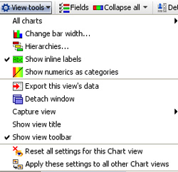
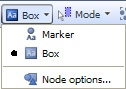
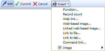
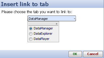
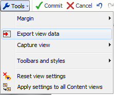
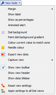
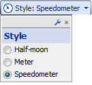
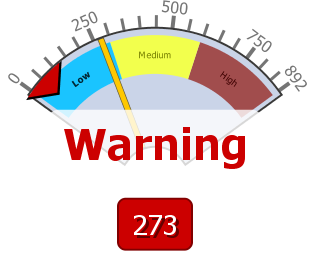
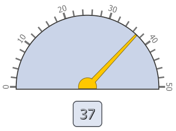
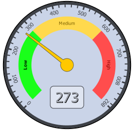
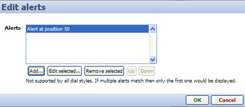
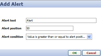
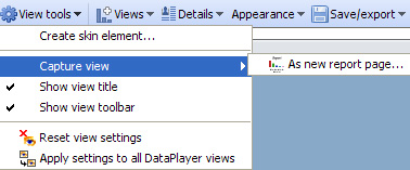
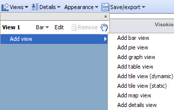
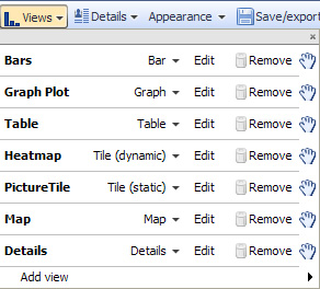
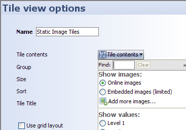
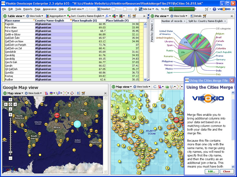
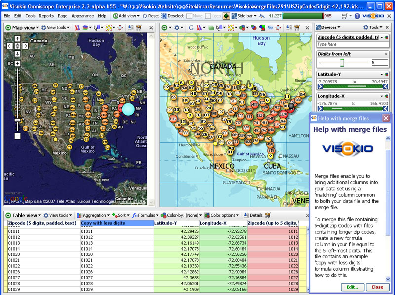
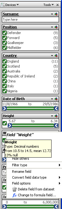
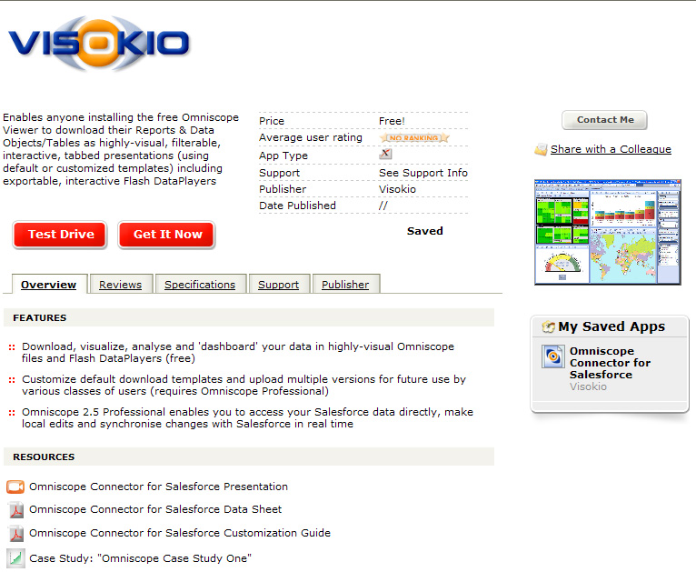
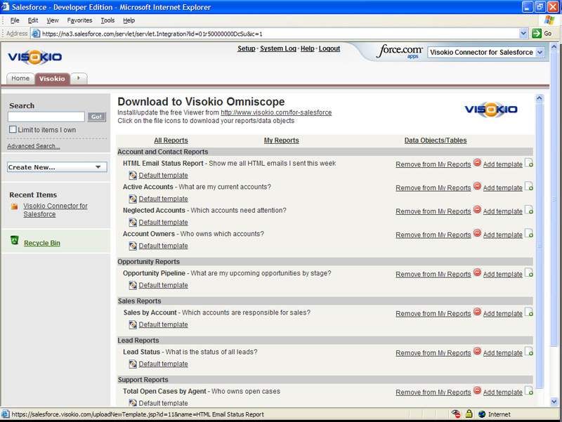

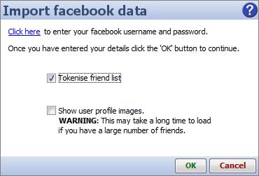
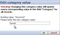
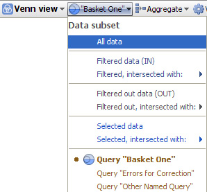
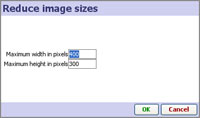

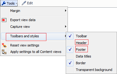
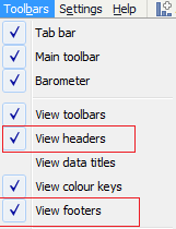
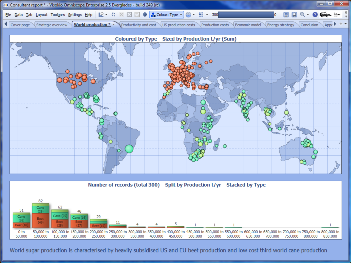
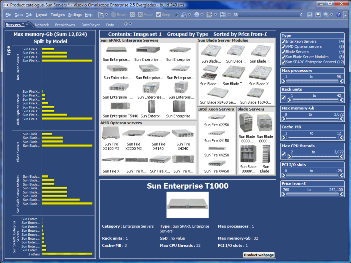
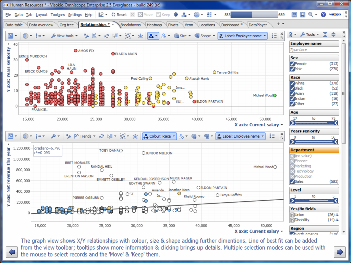
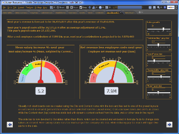
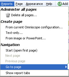


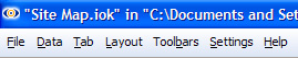
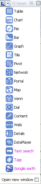
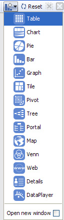

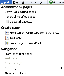
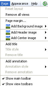
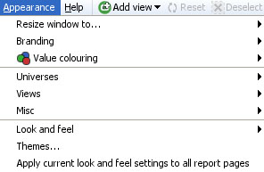
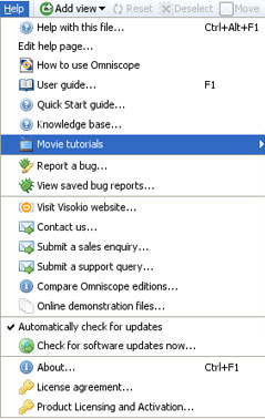
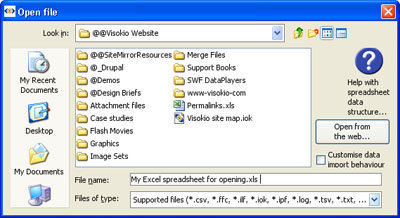
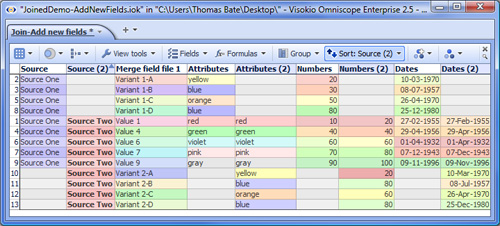
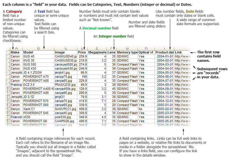